Free Statistics
of Irreproducible Research!
Description of Statistical Computation | |||||||||||||||||||||
|---|---|---|---|---|---|---|---|---|---|---|---|---|---|---|---|---|---|---|---|---|---|
| Author's title | |||||||||||||||||||||
| Author | *The author of this computation has been verified* | ||||||||||||||||||||
| R Software Module | rwasp_meanplot.wasp | ||||||||||||||||||||
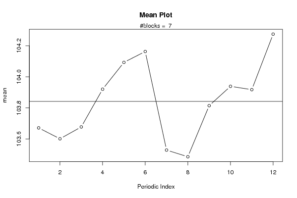
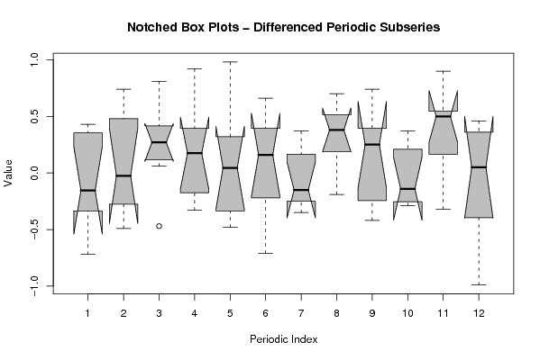
| Title produced by software | Mean Plot | ||||||||||||||||||||
| Date of computation | Fri, 31 Oct 2008 08:51:36 -0600 | ||||||||||||||||||||
| Cite this page as follows | Statistical Computations at FreeStatistics.org, Office for Research Development and Education, URL https://freestatistics.org/blog/index.php?v=date/2008/Oct/31/t12254647621adfw4ozgzm7j2p.htm/, Retrieved Wed, 15 May 2024 19:54:48 +0000 | ||||||||||||||||||||
| Statistical Computations at FreeStatistics.org, Office for Research Development and Education, URL https://freestatistics.org/blog/index.php?pk=20290, Retrieved Wed, 15 May 2024 19:54:48 +0000 | |||||||||||||||||||||
| QR Codes: | |||||||||||||||||||||
|
| |||||||||||||||||||||
| Original text written by user: | |||||||||||||||||||||
| IsPrivate? | No (this computation is public) | ||||||||||||||||||||
| User-defined keywords | |||||||||||||||||||||
| Estimated Impact | 161 | ||||||||||||||||||||
Tree of Dependent Computations | |||||||||||||||||||||
| Family? (F = Feedback message, R = changed R code, M = changed R Module, P = changed Parameters, D = changed Data) | |||||||||||||||||||||
| F [Mean Plot] [workshop 3] [2007-10-26 12:14:28] [e9ffc5de6f8a7be62f22b142b5b6b1a8] F D [Mean Plot] [taak 4 - Q2 Boxplot] [2008-10-30 12:55:29] [46c5a5fbda57fdfa1d4ef48658f82a0c] - R D [Mean Plot] [taak 4 part 2 Q3 ...] [2008-10-30 15:43:11] [46c5a5fbda57fdfa1d4ef48658f82a0c] F D [Mean Plot] [Q3 Hypothesis Tes...] [2008-10-31 14:51:36] [dbfa7caa6871c163dec68ca05d48bb00] [Current] | |||||||||||||||||||||
| Feedback Forum | |||||||||||||||||||||
Post a new message | |||||||||||||||||||||
Dataset | |||||||||||||||||||||
| Dataseries X: | |||||||||||||||||||||
100.00 100.39 100.15 100.21 100.03 99.58 99.40 99.77 100.41 100.12 99.83 99.73 98.74 98.44 98.79 99.60 99.82 99.85 100.01 100.28 100.63 101.14 101.51 102.41 102.46 102.09 101.99 101.52 102.44 103.42 103.63 103.28 103.98 103.56 103.42 103.92 103.81 103.09 102.60 102.77 102.60 102.88 102.17 101.85 101.66 101.91 102.13 102.71 103.17 102.89 102.94 103.33 103.75 104.11 104.77 104.62 105.00 105.74 105.94 106.37 106.65 107.08 106.77 107.21 107.34 107.12 106.86 106.92 106.95 107.23 106.94 106.62 105.94 105.91 106.52 106.85 107.22 107.28 107.86 107.68 108.07 107.87 107.65 108.16 108.60 108.92 109.66 109.87 109.54 109.06 | |||||||||||||||||||||
Tables (Output of Computation) | |||||||||||||||||||||
| |||||||||||||||||||||
Figures (Output of Computation) | |||||||||||||||||||||
Input Parameters & R Code | |||||||||||||||||||||
| Parameters (Session): | |||||||||||||||||||||
| par1 = 12 ; | |||||||||||||||||||||
| Parameters (R input): | |||||||||||||||||||||
| par1 = 12 ; | |||||||||||||||||||||
| R code (references can be found in the software module): | |||||||||||||||||||||
par1 <- as.numeric(par1) | |||||||||||||||||||||