Free Statistics
of Irreproducible Research!
Description of Statistical Computation | |||||||||||||||||||||
|---|---|---|---|---|---|---|---|---|---|---|---|---|---|---|---|---|---|---|---|---|---|
| Author's title | Seizoensinvloed en trends - Aantal geregistreerde domeinnamen - Dorien Dhan... | ||||||||||||||||||||
| Author | *Unverified author* | ||||||||||||||||||||
| R Software Module | rwasp_meanplot.wasp | ||||||||||||||||||||
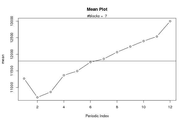
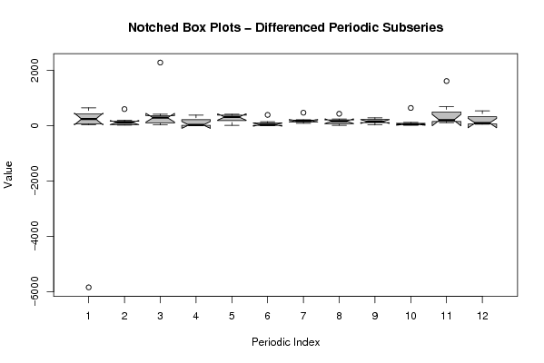
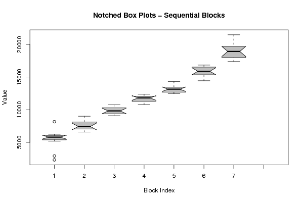
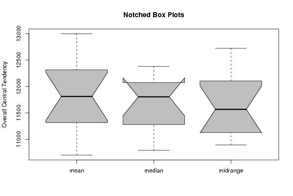
| Title produced by software | Mean Plot | ||||||||||||||||||||
| Date of computation | Thu, 23 Apr 2009 11:51:18 -0600 | ||||||||||||||||||||
| Cite this page as follows | Statistical Computations at FreeStatistics.org, Office for Research Development and Education, URL https://freestatistics.org/blog/index.php?v=date/2009/Apr/23/t124050913239x2iycz4gy5s2t.htm/, Retrieved Mon, 13 May 2024 08:07:57 +0000 | ||||||||||||||||||||
| Statistical Computations at FreeStatistics.org, Office for Research Development and Education, URL https://freestatistics.org/blog/index.php?pk=39347, Retrieved Mon, 13 May 2024 08:07:57 +0000 | |||||||||||||||||||||
| QR Codes: | |||||||||||||||||||||
|
| |||||||||||||||||||||
| Original text written by user: | |||||||||||||||||||||
| IsPrivate? | No (this computation is public) | ||||||||||||||||||||
| User-defined keywords | |||||||||||||||||||||
| Estimated Impact | 205 | ||||||||||||||||||||
Tree of Dependent Computations | |||||||||||||||||||||
| Family? (F = Feedback message, R = changed R code, M = changed R Module, P = changed Parameters, D = changed Data) | |||||||||||||||||||||
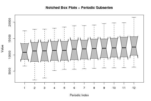
| - [Notched Boxplots] [Datareeks - Nieuw...] [2009-02-21 09:29:05] [74be16979710d4c4e7c6647856088456] - RMPD [Mean Plot] [Seizoensinvloed e...] [2009-04-23 17:51:18] [d41d8cd98f00b204e9800998ecf8427e] [Current] | |||||||||||||||||||||
| Feedback Forum | |||||||||||||||||||||
Post a new message | |||||||||||||||||||||
Dataset | |||||||||||||||||||||
| Dataseries X: | |||||||||||||||||||||
8166 2322 2924 5209 5597 5616 5764 5854 6019 6047 6082 6251 6576 6820 7024 7102 7107 7237 7630 7842 8086 8201 8323 9016 9077 9115 9230 9535 9565 9807 9815 9999 10176 10416 10439 10737 10790 11196 11221 11340 11356 11772 11836 11926 12013 12132 12178 12382 12448 12543 12662 12692 12767 13136 13145 13330 13381 13533 14176 14314 14444 15092 15130 15550 15557 15874 15892 16364 16379 16668 16713 16830 17368 17808 17846 18137 18504 18898 18938 19139 19573 19796 19845 21461 | |||||||||||||||||||||
Tables (Output of Computation) | |||||||||||||||||||||
| |||||||||||||||||||||
Figures (Output of Computation) | |||||||||||||||||||||
Input Parameters & R Code | |||||||||||||||||||||
| Parameters (Session): | |||||||||||||||||||||
| par1 = 12 ; | |||||||||||||||||||||
| Parameters (R input): | |||||||||||||||||||||
| par1 = 12 ; | |||||||||||||||||||||
| R code (references can be found in the software module): | |||||||||||||||||||||
par1 <- as.numeric(par1) | |||||||||||||||||||||