Free Statistics
of Irreproducible Research!
Description of Statistical Computation | |||||||||||||||||||||
|---|---|---|---|---|---|---|---|---|---|---|---|---|---|---|---|---|---|---|---|---|---|
| Author's title | Cijferreeks - Maandelijkse verkoop rode wijn mean plot - Renske van der Eij... | ||||||||||||||||||||
| Author | *Unverified author* | ||||||||||||||||||||
| R Software Module | rwasp_meanplot.wasp | ||||||||||||||||||||
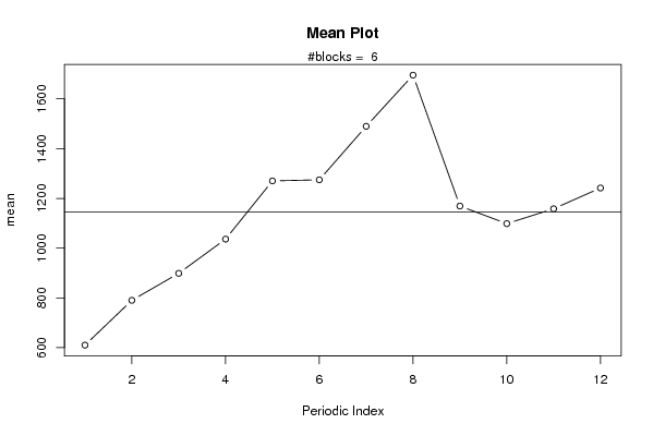
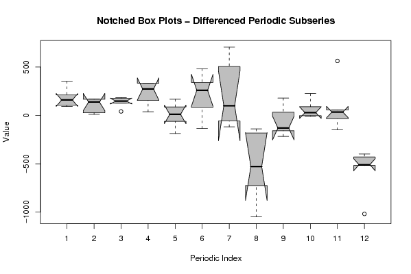
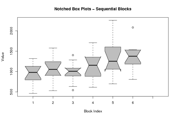
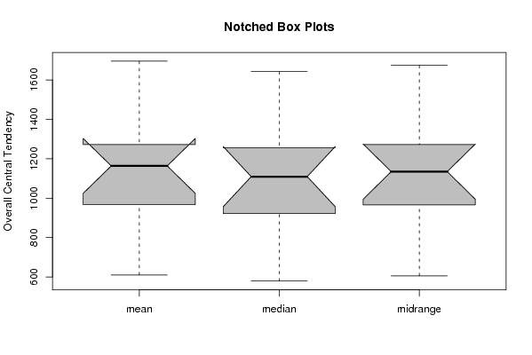
| Title produced by software | Mean Plot | ||||||||||||||||||||
| Date of computation | Thu, 30 Apr 2009 06:40:17 -0600 | ||||||||||||||||||||
| Cite this page as follows | Statistical Computations at FreeStatistics.org, Office for Research Development and Education, URL https://freestatistics.org/blog/index.php?v=date/2009/Apr/30/t1241095256m60duacha2mvgyn.htm/, Retrieved Sat, 11 May 2024 05:35:43 +0000 | ||||||||||||||||||||
| Statistical Computations at FreeStatistics.org, Office for Research Development and Education, URL https://freestatistics.org/blog/index.php?pk=39459, Retrieved Sat, 11 May 2024 05:35:43 +0000 | |||||||||||||||||||||
| QR Codes: | |||||||||||||||||||||
|
| |||||||||||||||||||||
| Original text written by user: | |||||||||||||||||||||
| IsPrivate? | No (this computation is public) | ||||||||||||||||||||
| User-defined keywords | |||||||||||||||||||||
| Estimated Impact | 240 | ||||||||||||||||||||
Tree of Dependent Computations | |||||||||||||||||||||
| Family? (F = Feedback message, R = changed R code, M = changed R Module, P = changed Parameters, D = changed Data) | |||||||||||||||||||||
| - [Univariate Data Series] [Cijferreeks - Maa...] [2009-04-30 12:38:22] [74be16979710d4c4e7c6647856088456] - RMP [Mean Plot] [Cijferreeks - Maa...] [2009-04-30 12:40:17] [d41d8cd98f00b204e9800998ecf8427e] [Current] | |||||||||||||||||||||
| Feedback Forum | |||||||||||||||||||||
Post a new message | |||||||||||||||||||||
Dataset | |||||||||||||||||||||
| Dataseries X: | |||||||||||||||||||||
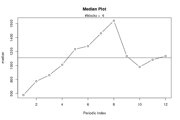
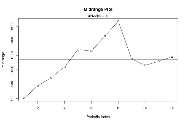
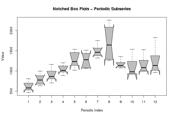
464 675 703 887 1139 1077 1318 1260 1120 963 996 960 530 883 894 1045 1199 1287 1565 1577 1076 918 1008 1063 544 635 804 980 1018 1064 1404 1286 1104 999 996 1015 615 722 832 977 1270 1437 1520 1708 1151 934 1159 1209 699 830 996 1124 1458 1270 1753 2258 1208 1241 1265 1828 809 997 1164 1205 1538 1513 1378 2083 1357 1536 1526 1376 | |||||||||||||||||||||
Tables (Output of Computation) | |||||||||||||||||||||
| |||||||||||||||||||||
Figures (Output of Computation) | |||||||||||||||||||||
Input Parameters & R Code | |||||||||||||||||||||
| Parameters (Session): | |||||||||||||||||||||
| par1 = 12 ; | |||||||||||||||||||||
| Parameters (R input): | |||||||||||||||||||||
| par1 = 12 ; | |||||||||||||||||||||
| R code (references can be found in the software module): | |||||||||||||||||||||
par1 <- as.numeric(par1) | |||||||||||||||||||||