Free Statistics
of Irreproducible Research!
Description of Statistical Computation | |||||||||||||||||||||
|---|---|---|---|---|---|---|---|---|---|---|---|---|---|---|---|---|---|---|---|---|---|
| Author's title | |||||||||||||||||||||
| Author | *The author of this computation has been verified* | ||||||||||||||||||||
| R Software Module | rwasp_meanplot.wasp | ||||||||||||||||||||
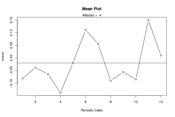
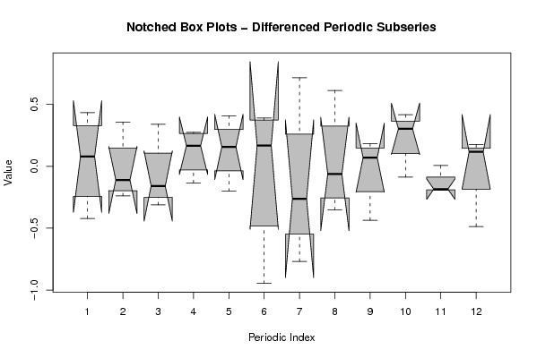
| Title produced by software | Mean Plot | ||||||||||||||||||||
| Date of computation | Wed, 02 Dec 2009 03:46:07 -0700 | ||||||||||||||||||||
| Cite this page as follows | Statistical Computations at FreeStatistics.org, Office for Research Development and Education, URL https://freestatistics.org/blog/index.php?v=date/2009/Dec/02/t1259750864mdsibgk80otecr4.htm/, Retrieved Sat, 27 Apr 2024 21:44:06 +0000 | ||||||||||||||||||||
| Statistical Computations at FreeStatistics.org, Office for Research Development and Education, URL https://freestatistics.org/blog/index.php?pk=62327, Retrieved Sat, 27 Apr 2024 21:44:06 +0000 | |||||||||||||||||||||
| QR Codes: | |||||||||||||||||||||
|
| |||||||||||||||||||||
| Original text written by user: | |||||||||||||||||||||
| IsPrivate? | No (this computation is public) | ||||||||||||||||||||
| User-defined keywords | cvm | ||||||||||||||||||||
| Estimated Impact | 173 | ||||||||||||||||||||
Tree of Dependent Computations | |||||||||||||||||||||
| Family? (F = Feedback message, R = changed R code, M = changed R Module, P = changed Parameters, D = changed Data) | |||||||||||||||||||||
| - [Univariate Data Series] [data set] [2008-12-01 19:54:57] [b98453cac15ba1066b407e146608df68] - RMP [ARIMA Backward Selection] [] [2009-11-27 14:53:14] [b98453cac15ba1066b407e146608df68] - D [ARIMA Backward Selection] [BBWS9-Arimabackward1] [2009-12-01 20:26:03] [408e92805dcb18620260f240a7fb9d53] - RM D [Harrell-Davis Quantiles] [BBWS9-Harolddavis] [2009-12-01 20:39:11] [408e92805dcb18620260f240a7fb9d53] - RM [Mean Plot] [BBWS9-Meanplot] [2009-12-01 20:43:16] [408e92805dcb18620260f240a7fb9d53] - PD [Mean Plot] [W9: Mean plot] [2009-12-02 10:46:07] [a5ada8bd39e806b5b90f09589c89554a] [Current] - D [Mean Plot] [WS9 Mean Plot Yt ...] [2009-12-04 16:04:10] [1b4c3bbe3f2ba180dd536c5a6a81a8e6] - D [Mean Plot] [W9.9] [2009-12-04 17:33:15] [d31db4f83c6a129f6d3e47077769e868] | |||||||||||||||||||||
| Feedback Forum | |||||||||||||||||||||
Post a new message | |||||||||||||||||||||
Dataset | |||||||||||||||||||||
| Dataseries X: | |||||||||||||||||||||
-0.0352348963249683 -0.0996886642707601 0.258351557360083 0.132707026411622 0.209190613791858 0.00765440528592697 0.364638644454261 -0.404729821174493 0.208323526616788 -0.228318339348579 0.0846424177144565 -0.108655058648595 0.00746541367547315 0.229284741496672 0.0735453904039185 -0.238534916960685 0.0362894953902089 0.163357762754455 0.141878886579970 -0.18679545624252 -0.151992074152852 -0.126522100160736 0.291127512736771 0.111350857781979 -0.375333748364419 0.0586735493662476 -0.00774453175246062 -0.201225232092894 0.0544700341223013 0.462862138244245 -0.483936137034753 0.230680122542856 -0.122800122937162 -0.00974091735299254 -0.0974876787295767 -0.0918746552479597 0.083000669337947 -0.338942397572222 -0.57777344126642 -0.239078710664643 -0.373618252683224 -0.188541466996174 0.200768061115737 0.00379888006595585 -0.155150788501183 0.0281973237494739 0.320159473131222 0.130359972235699 | |||||||||||||||||||||
Tables (Output of Computation) | |||||||||||||||||||||
| |||||||||||||||||||||
Figures (Output of Computation) | |||||||||||||||||||||
Input Parameters & R Code | |||||||||||||||||||||
| Parameters (Session): | |||||||||||||||||||||
| par1 = 12 ; | |||||||||||||||||||||
| Parameters (R input): | |||||||||||||||||||||
| par1 = 12 ; | |||||||||||||||||||||
| R code (references can be found in the software module): | |||||||||||||||||||||
par1 <- as.numeric(par1) | |||||||||||||||||||||