Repository of Reproducible Computations

Free Statistics

of Irreproducible Research!

Author's title

Author

*The author of this computation has been verified*

R Software Module

rwasp_autocorrelation.wasp

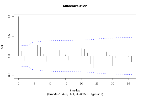
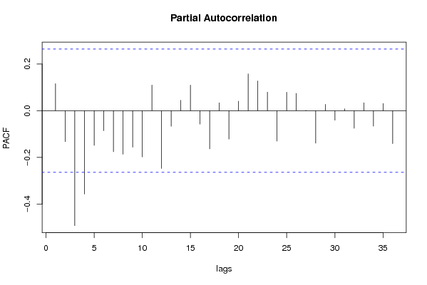
Title produced by software

(Partial) Autocorrelation Function

Date of computation

Wed, 02 Dec 2009 09:44:37 -0700

Cite this page as follows

Statistical Computations at FreeStatistics.org, Office for Research Development and Education, URL https://freestatistics.org/blog/index.php?v=date/2009/Dec/02/t1259772396ot3du5a2qb15rw8.htm/, Retrieved Sun, 28 Apr 2024 13:17:22 +0000

Statistical Computations at FreeStatistics.org, Office for Research Development and Education, URL https://freestatistics.org/blog/index.php?pk=62427, Retrieved Sun, 28 Apr 2024 13:17:22 +0000

QR Codes:

Paste this QR Code to cite your computation.

Original text written by user:

IsPrivate?

No (this computation is public)

User-defined keywords

Estimated Impact

185

Family? (F = Feedback message, R = changed R code, M = changed R Module, P = changed Parameters, D = changed Data)

-     [Univariate Data Series] [data set] [2008-12-01 19:54:57] [b98453cac15ba1066b407e146608df68]
- RMP   [(Partial) Autocorrelation Function] [] [2009-11-27 14:48:46] [b98453cac15ba1066b407e146608df68]
-   PD      [(Partial) Autocorrelation Function] [ACF (d = 2, D = 1)] [2009-12-02 16:44:37] [acc980be4047884b6edd254cd7beb9fa] [Current]
-   P         [(Partial) Autocorrelation Function] [ACF (d = 1, D = 0)] [2009-12-02 19:32:48] [ee7c2e7343f5b1451e62c5c16ec521f1] 
- R PD          [(Partial) Autocorrelation Function] [d = D = 1] [2009-12-03 22:05:10] [a6a5b7f2bf4260cfaf90c3e1a175c944] 
-   P             [(Partial) Autocorrelation Function] [(partial) autocor...] [2009-12-13 16:20:38] [a6a5b7f2bf4260cfaf90c3e1a175c944] 
-               [(Partial) Autocorrelation Function] [] [2009-12-04 21:31:38] [859f65298c93b90426725427c75f8582] 
-    D            [(Partial) Autocorrelation Function] [] [2009-12-20 18:41:02] [a3c75f2af6eea9d676b2dadad1cedbf1] 
-               [(Partial) Autocorrelation Function] [] [2009-12-13 10:40:28] [b7349fb284cae6f1172638396d27b11f] 

Feedback Forum

Post a new message

Dataseries X:

Download CSV

Histogram

Boxplots

8.2
8
7.5
6.8
6.5
6.6
7.6
8
8.1
7.7
7.5
7.6
7.8
7.8
7.8
7.5
7.5
7.1
7.5
7.5
7.6
7.7
7.7
7.9
8.1
8.2
8.2
8.2
7.9
7.3
6.9
6.6
6.7
6.9
7
7.1
7.2
7.1
6.9
7
6.8
6.4
6.7
6.6
6.4
6.3
6.2
6.5
6.8
6.8
6.4
6.1
5.8
6.1
7.2
7.3
6.9
6.1
5.8
6.2
7.1
7.7
7.9
7.7
7.4
7.5
8
8.1
8

Summary of computational transaction
Raw Input	view raw input (R code)
Raw Output	view raw output of R engine
Computing time	1 seconds
R Server	'Gwilym Jenkins' @ 72.249.127.135

\begin{tabular}{lllllllll}
\hline
Summary of computational transaction \tabularnewline
Raw Input & view raw input (R code)  \tabularnewline
Raw Output & view raw output of R engine  \tabularnewline
Computing time & 1 seconds \tabularnewline
R Server & 'Gwilym Jenkins' @ 72.249.127.135 \tabularnewline
\hline
\end{tabular}
%Source: https://freestatistics.org/blog/index.php?pk=62427&T=0

[TABLE]
[ROW][C]Summary of computational transaction[/C][/ROW]
[ROW][C]Raw Input[/C][C]view raw input (R code) [/C][/ROW]
[ROW][C]Raw Output[/C][C]view raw output of R engine [/C][/ROW]
[ROW][C]Computing time[/C][C]1 seconds[/C][/ROW]
[ROW][C]R Server[/C][C]'Gwilym Jenkins' @ 72.249.127.135[/C][/ROW]
[/TABLE]
Source: https://freestatistics.org/blog/index.php?pk=62427&T=0

Globally Unique Identifier (entire table): ba.freestatistics.org/blog/index.php?pk=62427&T=0

As an alternative you can also use a QR Code:

The GUIDs for individual cells are displayed in the table below:

Summary of computational transaction
Raw Input	view raw input (R code)
Raw Output	view raw output of R engine
Computing time	1 seconds
R Server	'Gwilym Jenkins' @ 72.249.127.135

Autocorrelation Function
Time lag k	ACF(k)	T-STAT	P-value
1	0.116037	0.8606	0.196611
2	-0.117119	-0.8686	0.194427
3	-0.508052	-3.7678	0.000202
4	-0.344871	-2.5576	0.006663
5	0.00278	0.0206	0.491812
6	0.273137	2.0256	0.023832
7	0.228667	1.6958	0.047785
8	0.040089	0.2973	0.383676
9	-0.139654	-1.0357	0.152436
10	-0.184178	-1.3659	0.088764
11	0.117572	0.8719	0.193517
12	-0.041531	-0.308	0.379623
13	0.139616	1.0354	0.152501
14	0.004316	0.032	0.487291
15	0.030927	0.2294	0.40972
16	-0.108507	-0.8047	0.212225
17	-0.130878	-0.9706	0.167995
18	-0.011923	-0.0884	0.46493
19	0.004421	0.0328	0.48698
20	0.188676	1.3993	0.083676
21	0.176788	1.3111	0.097637
22	0.080256	0.5952	0.277077
23	-0.209473	-1.5535	0.063021
24	-0.309057	-2.292	0.012878
25	-0.116022	-0.8604	0.196639
26	0.164763	1.2219	0.113476
27	0.237708	1.7629	0.041738
28	0.108486	0.8046	0.212271
29	0.009063	0.0672	0.473327
30	-0.254	-1.8837	0.032447
31	-0.04462	-0.3309	0.370985
32	-0.011957	-0.0887	0.464831
33	0.200557	1.4874	0.071314
34	0.002982	0.0221	0.491218
35	-0.026737	-0.1983	0.421776
36	-0.147097	-1.0909	0.140036

\begin{tabular}{lllllllll}
\hline
Autocorrelation Function \tabularnewline
Time lag k & ACF(k) & T-STAT & P-value \tabularnewline
1 & 0.116037 & 0.8606 & 0.196611 \tabularnewline
2 & -0.117119 & -0.8686 & 0.194427 \tabularnewline
3 & -0.508052 & -3.7678 & 0.000202 \tabularnewline
4 & -0.344871 & -2.5576 & 0.006663 \tabularnewline
5 & 0.00278 & 0.0206 & 0.491812 \tabularnewline
6 & 0.273137 & 2.0256 & 0.023832 \tabularnewline
7 & 0.228667 & 1.6958 & 0.047785 \tabularnewline
8 & 0.040089 & 0.2973 & 0.383676 \tabularnewline
9 & -0.139654 & -1.0357 & 0.152436 \tabularnewline
10 & -0.184178 & -1.3659 & 0.088764 \tabularnewline
11 & 0.117572 & 0.8719 & 0.193517 \tabularnewline
12 & -0.041531 & -0.308 & 0.379623 \tabularnewline
13 & 0.139616 & 1.0354 & 0.152501 \tabularnewline
14 & 0.004316 & 0.032 & 0.487291 \tabularnewline
15 & 0.030927 & 0.2294 & 0.40972 \tabularnewline
16 & -0.108507 & -0.8047 & 0.212225 \tabularnewline
17 & -0.130878 & -0.9706 & 0.167995 \tabularnewline
18 & -0.011923 & -0.0884 & 0.46493 \tabularnewline
19 & 0.004421 & 0.0328 & 0.48698 \tabularnewline
20 & 0.188676 & 1.3993 & 0.083676 \tabularnewline
21 & 0.176788 & 1.3111 & 0.097637 \tabularnewline
22 & 0.080256 & 0.5952 & 0.277077 \tabularnewline
23 & -0.209473 & -1.5535 & 0.063021 \tabularnewline
24 & -0.309057 & -2.292 & 0.012878 \tabularnewline
25 & -0.116022 & -0.8604 & 0.196639 \tabularnewline
26 & 0.164763 & 1.2219 & 0.113476 \tabularnewline
27 & 0.237708 & 1.7629 & 0.041738 \tabularnewline
28 & 0.108486 & 0.8046 & 0.212271 \tabularnewline
29 & 0.009063 & 0.0672 & 0.473327 \tabularnewline
30 & -0.254 & -1.8837 & 0.032447 \tabularnewline
31 & -0.04462 & -0.3309 & 0.370985 \tabularnewline
32 & -0.011957 & -0.0887 & 0.464831 \tabularnewline
33 & 0.200557 & 1.4874 & 0.071314 \tabularnewline
34 & 0.002982 & 0.0221 & 0.491218 \tabularnewline
35 & -0.026737 & -0.1983 & 0.421776 \tabularnewline
36 & -0.147097 & -1.0909 & 0.140036 \tabularnewline
\hline
\end{tabular}
%Source: https://freestatistics.org/blog/index.php?pk=62427&T=1

[TABLE]
[ROW][C]Autocorrelation Function[/C][/ROW]
[ROW][C]Time lag k[/C][C]ACF(k)[/C][C]T-STAT[/C][C]P-value[/C][/ROW]
[ROW][C]1[/C][C]0.116037[/C][C]0.8606[/C][C]0.196611[/C][/ROW]
[ROW][C]2[/C][C]-0.117119[/C][C]-0.8686[/C][C]0.194427[/C][/ROW]
[ROW][C]3[/C][C]-0.508052[/C][C]-3.7678[/C][C]0.000202[/C][/ROW]
[ROW][C]4[/C][C]-0.344871[/C][C]-2.5576[/C][C]0.006663[/C][/ROW]
[ROW][C]5[/C][C]0.00278[/C][C]0.0206[/C][C]0.491812[/C][/ROW]
[ROW][C]6[/C][C]0.273137[/C][C]2.0256[/C][C]0.023832[/C][/ROW]
[ROW][C]7[/C][C]0.228667[/C][C]1.6958[/C][C]0.047785[/C][/ROW]
[ROW][C]8[/C][C]0.040089[/C][C]0.2973[/C][C]0.383676[/C][/ROW]
[ROW][C]9[/C][C]-0.139654[/C][C]-1.0357[/C][C]0.152436[/C][/ROW]
[ROW][C]10[/C][C]-0.184178[/C][C]-1.3659[/C][C]0.088764[/C][/ROW]
[ROW][C]11[/C][C]0.117572[/C][C]0.8719[/C][C]0.193517[/C][/ROW]
[ROW][C]12[/C][C]-0.041531[/C][C]-0.308[/C][C]0.379623[/C][/ROW]
[ROW][C]13[/C][C]0.139616[/C][C]1.0354[/C][C]0.152501[/C][/ROW]
[ROW][C]14[/C][C]0.004316[/C][C]0.032[/C][C]0.487291[/C][/ROW]
[ROW][C]15[/C][C]0.030927[/C][C]0.2294[/C][C]0.40972[/C][/ROW]
[ROW][C]16[/C][C]-0.108507[/C][C]-0.8047[/C][C]0.212225[/C][/ROW]
[ROW][C]17[/C][C]-0.130878[/C][C]-0.9706[/C][C]0.167995[/C][/ROW]
[ROW][C]18[/C][C]-0.011923[/C][C]-0.0884[/C][C]0.46493[/C][/ROW]
[ROW][C]19[/C][C]0.004421[/C][C]0.0328[/C][C]0.48698[/C][/ROW]
[ROW][C]20[/C][C]0.188676[/C][C]1.3993[/C][C]0.083676[/C][/ROW]
[ROW][C]21[/C][C]0.176788[/C][C]1.3111[/C][C]0.097637[/C][/ROW]
[ROW][C]22[/C][C]0.080256[/C][C]0.5952[/C][C]0.277077[/C][/ROW]
[ROW][C]23[/C][C]-0.209473[/C][C]-1.5535[/C][C]0.063021[/C][/ROW]
[ROW][C]24[/C][C]-0.309057[/C][C]-2.292[/C][C]0.012878[/C][/ROW]
[ROW][C]25[/C][C]-0.116022[/C][C]-0.8604[/C][C]0.196639[/C][/ROW]
[ROW][C]26[/C][C]0.164763[/C][C]1.2219[/C][C]0.113476[/C][/ROW]
[ROW][C]27[/C][C]0.237708[/C][C]1.7629[/C][C]0.041738[/C][/ROW]
[ROW][C]28[/C][C]0.108486[/C][C]0.8046[/C][C]0.212271[/C][/ROW]
[ROW][C]29[/C][C]0.009063[/C][C]0.0672[/C][C]0.473327[/C][/ROW]
[ROW][C]30[/C][C]-0.254[/C][C]-1.8837[/C][C]0.032447[/C][/ROW]
[ROW][C]31[/C][C]-0.04462[/C][C]-0.3309[/C][C]0.370985[/C][/ROW]
[ROW][C]32[/C][C]-0.011957[/C][C]-0.0887[/C][C]0.464831[/C][/ROW]
[ROW][C]33[/C][C]0.200557[/C][C]1.4874[/C][C]0.071314[/C][/ROW]
[ROW][C]34[/C][C]0.002982[/C][C]0.0221[/C][C]0.491218[/C][/ROW]
[ROW][C]35[/C][C]-0.026737[/C][C]-0.1983[/C][C]0.421776[/C][/ROW]
[ROW][C]36[/C][C]-0.147097[/C][C]-1.0909[/C][C]0.140036[/C][/ROW]
[/TABLE]
Source: https://freestatistics.org/blog/index.php?pk=62427&T=1

Globally Unique Identifier (entire table): ba.freestatistics.org/blog/index.php?pk=62427&T=1

As an alternative you can also use a QR Code:

The GUIDs for individual cells are displayed in the table below:

Autocorrelation Function
Time lag k	ACF(k)	T-STAT	P-value
1	0.116037	0.8606	0.196611
2	-0.117119	-0.8686	0.194427
3	-0.508052	-3.7678	0.000202
4	-0.344871	-2.5576	0.006663
5	0.00278	0.0206	0.491812
6	0.273137	2.0256	0.023832
7	0.228667	1.6958	0.047785
8	0.040089	0.2973	0.383676
9	-0.139654	-1.0357	0.152436
10	-0.184178	-1.3659	0.088764
11	0.117572	0.8719	0.193517
12	-0.041531	-0.308	0.379623
13	0.139616	1.0354	0.152501
14	0.004316	0.032	0.487291
15	0.030927	0.2294	0.40972
16	-0.108507	-0.8047	0.212225
17	-0.130878	-0.9706	0.167995
18	-0.011923	-0.0884	0.46493
19	0.004421	0.0328	0.48698
20	0.188676	1.3993	0.083676
21	0.176788	1.3111	0.097637
22	0.080256	0.5952	0.277077
23	-0.209473	-1.5535	0.063021
24	-0.309057	-2.292	0.012878
25	-0.116022	-0.8604	0.196639
26	0.164763	1.2219	0.113476
27	0.237708	1.7629	0.041738
28	0.108486	0.8046	0.212271
29	0.009063	0.0672	0.473327
30	-0.254	-1.8837	0.032447
31	-0.04462	-0.3309	0.370985
32	-0.011957	-0.0887	0.464831
33	0.200557	1.4874	0.071314
34	0.002982	0.0221	0.491218
35	-0.026737	-0.1983	0.421776
36	-0.147097	-1.0909	0.140036

Partial Autocorrelation Function
Time lag k	PACF(k)	T-STAT	P-value
1	0.116037	0.8606	0.196611
2	-0.132366	-0.9816	0.165286
3	-0.492447	-3.6521	0.00029
4	-0.356868	-2.6466	0.005292
5	-0.148481	-1.1012	0.13781
6	-0.08564	-0.6351	0.263991
7	-0.175636	-1.3025	0.099079
8	-0.186368	-1.3821	0.086258
9	-0.156087	-1.1576	0.12602
10	-0.197664	-1.4659	0.074183
11	0.1099	0.815	0.209282
12	-0.247466	-1.8353	0.035938
13	-0.06625	-0.4913	0.312577
14	0.044681	0.3314	0.370815
15	0.110142	0.8168	0.208773
16	-0.057133	-0.4237	0.336716
17	-0.163305	-1.2111	0.115517
18	0.034244	0.254	0.400236
19	-0.121304	-0.8996	0.186123
20	0.040804	0.3026	0.381665
21	0.15819	1.1732	0.122892
22	0.127946	0.9489	0.173418
23	0.080025	0.5935	0.277645
24	-0.130051	-0.9645	0.169512
25	0.079408	0.5889	0.279168
26	0.074505	0.5525	0.291406
27	0.002016	0.0149	0.494064
28	-0.139038	-1.0311	0.153496
29	0.027485	0.2038	0.419617
30	-0.040509	-0.3004	0.382494
31	0.00813	0.0603	0.476069
32	-0.075023	-0.5564	0.290102
33	0.03427	0.2542	0.400162
34	-0.065889	-0.4886	0.313518
35	0.030924	0.2293	0.409729
36	-0.140754	-1.0439	0.150558

\begin{tabular}{lllllllll}
\hline
Partial Autocorrelation Function \tabularnewline
Time lag k & PACF(k) & T-STAT & P-value \tabularnewline
1 & 0.116037 & 0.8606 & 0.196611 \tabularnewline
2 & -0.132366 & -0.9816 & 0.165286 \tabularnewline
3 & -0.492447 & -3.6521 & 0.00029 \tabularnewline
4 & -0.356868 & -2.6466 & 0.005292 \tabularnewline
5 & -0.148481 & -1.1012 & 0.13781 \tabularnewline
6 & -0.08564 & -0.6351 & 0.263991 \tabularnewline
7 & -0.175636 & -1.3025 & 0.099079 \tabularnewline
8 & -0.186368 & -1.3821 & 0.086258 \tabularnewline
9 & -0.156087 & -1.1576 & 0.12602 \tabularnewline
10 & -0.197664 & -1.4659 & 0.074183 \tabularnewline
11 & 0.1099 & 0.815 & 0.209282 \tabularnewline
12 & -0.247466 & -1.8353 & 0.035938 \tabularnewline
13 & -0.06625 & -0.4913 & 0.312577 \tabularnewline
14 & 0.044681 & 0.3314 & 0.370815 \tabularnewline
15 & 0.110142 & 0.8168 & 0.208773 \tabularnewline
16 & -0.057133 & -0.4237 & 0.336716 \tabularnewline
17 & -0.163305 & -1.2111 & 0.115517 \tabularnewline
18 & 0.034244 & 0.254 & 0.400236 \tabularnewline
19 & -0.121304 & -0.8996 & 0.186123 \tabularnewline
20 & 0.040804 & 0.3026 & 0.381665 \tabularnewline
21 & 0.15819 & 1.1732 & 0.122892 \tabularnewline
22 & 0.127946 & 0.9489 & 0.173418 \tabularnewline
23 & 0.080025 & 0.5935 & 0.277645 \tabularnewline
24 & -0.130051 & -0.9645 & 0.169512 \tabularnewline
25 & 0.079408 & 0.5889 & 0.279168 \tabularnewline
26 & 0.074505 & 0.5525 & 0.291406 \tabularnewline
27 & 0.002016 & 0.0149 & 0.494064 \tabularnewline
28 & -0.139038 & -1.0311 & 0.153496 \tabularnewline
29 & 0.027485 & 0.2038 & 0.419617 \tabularnewline
30 & -0.040509 & -0.3004 & 0.382494 \tabularnewline
31 & 0.00813 & 0.0603 & 0.476069 \tabularnewline
32 & -0.075023 & -0.5564 & 0.290102 \tabularnewline
33 & 0.03427 & 0.2542 & 0.400162 \tabularnewline
34 & -0.065889 & -0.4886 & 0.313518 \tabularnewline
35 & 0.030924 & 0.2293 & 0.409729 \tabularnewline
36 & -0.140754 & -1.0439 & 0.150558 \tabularnewline
\hline
\end{tabular}
%Source: https://freestatistics.org/blog/index.php?pk=62427&T=2

[TABLE]
[ROW][C]Partial Autocorrelation Function[/C][/ROW]
[ROW][C]Time lag k[/C][C]PACF(k)[/C][C]T-STAT[/C][C]P-value[/C][/ROW]
[ROW][C]1[/C][C]0.116037[/C][C]0.8606[/C][C]0.196611[/C][/ROW]
[ROW][C]2[/C][C]-0.132366[/C][C]-0.9816[/C][C]0.165286[/C][/ROW]
[ROW][C]3[/C][C]-0.492447[/C][C]-3.6521[/C][C]0.00029[/C][/ROW]
[ROW][C]4[/C][C]-0.356868[/C][C]-2.6466[/C][C]0.005292[/C][/ROW]
[ROW][C]5[/C][C]-0.148481[/C][C]-1.1012[/C][C]0.13781[/C][/ROW]
[ROW][C]6[/C][C]-0.08564[/C][C]-0.6351[/C][C]0.263991[/C][/ROW]
[ROW][C]7[/C][C]-0.175636[/C][C]-1.3025[/C][C]0.099079[/C][/ROW]
[ROW][C]8[/C][C]-0.186368[/C][C]-1.3821[/C][C]0.086258[/C][/ROW]
[ROW][C]9[/C][C]-0.156087[/C][C]-1.1576[/C][C]0.12602[/C][/ROW]
[ROW][C]10[/C][C]-0.197664[/C][C]-1.4659[/C][C]0.074183[/C][/ROW]
[ROW][C]11[/C][C]0.1099[/C][C]0.815[/C][C]0.209282[/C][/ROW]
[ROW][C]12[/C][C]-0.247466[/C][C]-1.8353[/C][C]0.035938[/C][/ROW]
[ROW][C]13[/C][C]-0.06625[/C][C]-0.4913[/C][C]0.312577[/C][/ROW]
[ROW][C]14[/C][C]0.044681[/C][C]0.3314[/C][C]0.370815[/C][/ROW]
[ROW][C]15[/C][C]0.110142[/C][C]0.8168[/C][C]0.208773[/C][/ROW]
[ROW][C]16[/C][C]-0.057133[/C][C]-0.4237[/C][C]0.336716[/C][/ROW]
[ROW][C]17[/C][C]-0.163305[/C][C]-1.2111[/C][C]0.115517[/C][/ROW]
[ROW][C]18[/C][C]0.034244[/C][C]0.254[/C][C]0.400236[/C][/ROW]
[ROW][C]19[/C][C]-0.121304[/C][C]-0.8996[/C][C]0.186123[/C][/ROW]
[ROW][C]20[/C][C]0.040804[/C][C]0.3026[/C][C]0.381665[/C][/ROW]
[ROW][C]21[/C][C]0.15819[/C][C]1.1732[/C][C]0.122892[/C][/ROW]
[ROW][C]22[/C][C]0.127946[/C][C]0.9489[/C][C]0.173418[/C][/ROW]
[ROW][C]23[/C][C]0.080025[/C][C]0.5935[/C][C]0.277645[/C][/ROW]
[ROW][C]24[/C][C]-0.130051[/C][C]-0.9645[/C][C]0.169512[/C][/ROW]
[ROW][C]25[/C][C]0.079408[/C][C]0.5889[/C][C]0.279168[/C][/ROW]
[ROW][C]26[/C][C]0.074505[/C][C]0.5525[/C][C]0.291406[/C][/ROW]
[ROW][C]27[/C][C]0.002016[/C][C]0.0149[/C][C]0.494064[/C][/ROW]
[ROW][C]28[/C][C]-0.139038[/C][C]-1.0311[/C][C]0.153496[/C][/ROW]
[ROW][C]29[/C][C]0.027485[/C][C]0.2038[/C][C]0.419617[/C][/ROW]
[ROW][C]30[/C][C]-0.040509[/C][C]-0.3004[/C][C]0.382494[/C][/ROW]
[ROW][C]31[/C][C]0.00813[/C][C]0.0603[/C][C]0.476069[/C][/ROW]
[ROW][C]32[/C][C]-0.075023[/C][C]-0.5564[/C][C]0.290102[/C][/ROW]
[ROW][C]33[/C][C]0.03427[/C][C]0.2542[/C][C]0.400162[/C][/ROW]
[ROW][C]34[/C][C]-0.065889[/C][C]-0.4886[/C][C]0.313518[/C][/ROW]
[ROW][C]35[/C][C]0.030924[/C][C]0.2293[/C][C]0.409729[/C][/ROW]
[ROW][C]36[/C][C]-0.140754[/C][C]-1.0439[/C][C]0.150558[/C][/ROW]
[/TABLE]
Source: https://freestatistics.org/blog/index.php?pk=62427&T=2

Globally Unique Identifier (entire table): ba.freestatistics.org/blog/index.php?pk=62427&T=2

As an alternative you can also use a QR Code:

The GUIDs for individual cells are displayed in the table below:

Partial Autocorrelation Function
Time lag k	PACF(k)	T-STAT	P-value
1	0.116037	0.8606	0.196611
2	-0.132366	-0.9816	0.165286
3	-0.492447	-3.6521	0.00029
4	-0.356868	-2.6466	0.005292
5	-0.148481	-1.1012	0.13781
6	-0.08564	-0.6351	0.263991
7	-0.175636	-1.3025	0.099079
8	-0.186368	-1.3821	0.086258
9	-0.156087	-1.1576	0.12602
10	-0.197664	-1.4659	0.074183
11	0.1099	0.815	0.209282
12	-0.247466	-1.8353	0.035938
13	-0.06625	-0.4913	0.312577
14	0.044681	0.3314	0.370815
15	0.110142	0.8168	0.208773
16	-0.057133	-0.4237	0.336716
17	-0.163305	-1.2111	0.115517
18	0.034244	0.254	0.400236
19	-0.121304	-0.8996	0.186123
20	0.040804	0.3026	0.381665
21	0.15819	1.1732	0.122892
22	0.127946	0.9489	0.173418
23	0.080025	0.5935	0.277645
24	-0.130051	-0.9645	0.169512
25	0.079408	0.5889	0.279168
26	0.074505	0.5525	0.291406
27	0.002016	0.0149	0.494064
28	-0.139038	-1.0311	0.153496
29	0.027485	0.2038	0.419617
30	-0.040509	-0.3004	0.382494
31	0.00813	0.0603	0.476069
32	-0.075023	-0.5564	0.290102
33	0.03427	0.2542	0.400162
34	-0.065889	-0.4886	0.313518
35	0.030924	0.2293	0.409729
36	-0.140754	-1.0439	0.150558

Figure 1

PNG link

Postscript link

PDF link

Figure 2

PNG link

Postscript link

PDF link

Parameters (Session):

par1 = 36 ; par2 = 1 ; par3 = 2 ; par4 = 1 ; par5 = 12 ; par6 = MA ; par7 = 0.95 ;

Parameters (R input):

par1 = 36 ; par2 = 1 ; par3 = 2 ; par4 = 1 ; par5 = 12 ; par6 = MA ; par7 = 0.95 ;

R code (references can be found in the software module):

if (par1 == 'Default') {
par1 = 10*log10(length(x))
} else {
par1 <- as.numeric(par1)
}
par2 <- as.numeric(par2)
par3 <- as.numeric(par3)
par4 <- as.numeric(par4)
par5 <- as.numeric(par5)
if (par6 == 'White Noise') par6 <- 'white' else par6 <- 'ma'
par7 <- as.numeric(par7)
if (par2 == 0) {
x <- log(x)
} else {
x <- (x ^ par2 - 1) / par2
}
if (par3 > 0) x <- diff(x,lag=1,difference=par3)
if (par4 > 0) x <- diff(x,lag=par5,difference=par4)
bitmap(file='pic1.png')
racf <- acf(x, par1, main='Autocorrelation', xlab='time lag', ylab='ACF', ci.type=par6, ci=par7, sub=paste('(lambda=',par2,', d=',par3,', D=',par4,', CI=', par7, ', CI type=',par6,')',sep=''))
dev.off()
bitmap(file='pic2.png')
rpacf <- pacf(x,par1,main='Partial Autocorrelation',xlab='lags',ylab='PACF')
dev.off()
(myacf <- c(racf$acf))
(mypacf <- c(rpacf$acf))
lengthx <- length(x)
sqrtn <- sqrt(lengthx)
load(file='createtable')
a<-table.start()
a<-table.row.start(a)
a<-table.element(a,'Autocorrelation Function',4,TRUE)
a<-table.row.end(a)
a<-table.row.start(a)
a<-table.element(a,'Time lag k',header=TRUE)
a<-table.element(a,hyperlink('basics.htm','ACF(k)','click here for more information about the Autocorrelation Function'),header=TRUE)
a<-table.element(a,'T-STAT',header=TRUE)
a<-table.element(a,'P-value',header=TRUE)
a<-table.row.end(a)
for (i in 2:(par1+1)) {
a<-table.row.start(a)
a<-table.element(a,i-1,header=TRUE)
a<-table.element(a,round(myacf[i],6))
mytstat <- myacf[i]*sqrtn
a<-table.element(a,round(mytstat,4))
a<-table.element(a,round(1-pt(abs(mytstat),lengthx),6))
a<-table.row.end(a)
}
a<-table.end(a)
table.save(a,file='mytable.tab')
a<-table.start()
a<-table.row.start(a)
a<-table.element(a,'Partial Autocorrelation Function',4,TRUE)
a<-table.row.end(a)
a<-table.row.start(a)
a<-table.element(a,'Time lag k',header=TRUE)
a<-table.element(a,hyperlink('basics.htm','PACF(k)','click here for more information about the Partial Autocorrelation Function'),header=TRUE)
a<-table.element(a,'T-STAT',header=TRUE)
a<-table.element(a,'P-value',header=TRUE)
a<-table.row.end(a)
for (i in 1:par1) {
a<-table.row.start(a)
a<-table.element(a,i,header=TRUE)
a<-table.element(a,round(mypacf[i],6))
mytstat <- mypacf[i]*sqrtn
a<-table.element(a,round(mytstat,4))
a<-table.element(a,round(1-pt(abs(mytstat),lengthx),6))
a<-table.row.end(a)
}
a<-table.end(a)
table.save(a,file='mytable1.tab')

Free Statistics

Description of Statistical Computation

Tree of Dependent Computations

Dataset

Tables (Output of Computation)

Figures (Output of Computation)

Input Parameters & R Code