Free Statistics
of Irreproducible Research!
Description of Statistical Computation | |||||||||||||||||||||
|---|---|---|---|---|---|---|---|---|---|---|---|---|---|---|---|---|---|---|---|---|---|
| Author's title | |||||||||||||||||||||
| Author | *The author of this computation has been verified* | ||||||||||||||||||||
| R Software Module | rwasp_meanplot.wasp | ||||||||||||||||||||
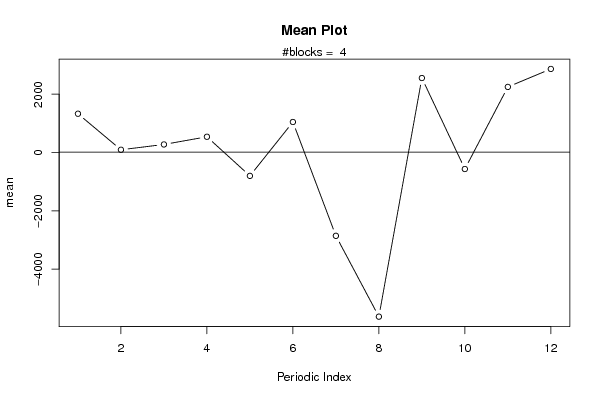
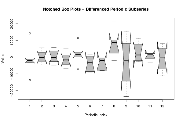
| Title produced by software | Mean Plot | ||||||||||||||||||||
| Date of computation | Wed, 02 Dec 2009 14:29:27 -0700 | ||||||||||||||||||||
| Cite this page as follows | Statistical Computations at FreeStatistics.org, Office for Research Development and Education, URL https://freestatistics.org/blog/index.php?v=date/2009/Dec/02/t1259789508yf3kbipw37t11kx.htm/, Retrieved Sun, 28 Apr 2024 10:32:19 +0000 | ||||||||||||||||||||
| Statistical Computations at FreeStatistics.org, Office for Research Development and Education, URL https://freestatistics.org/blog/index.php?pk=62598, Retrieved Sun, 28 Apr 2024 10:32:19 +0000 | |||||||||||||||||||||
| QR Codes: | |||||||||||||||||||||
|
| |||||||||||||||||||||
| Original text written by user: | |||||||||||||||||||||
| IsPrivate? | No (this computation is public) | ||||||||||||||||||||
| User-defined keywords | |||||||||||||||||||||
| Estimated Impact | 124 | ||||||||||||||||||||
Tree of Dependent Computations | |||||||||||||||||||||
| Family? (F = Feedback message, R = changed R code, M = changed R Module, P = changed Parameters, D = changed Data) | |||||||||||||||||||||
| - [Univariate Data Series] [data set] [2008-12-01 19:54:57] [b98453cac15ba1066b407e146608df68] - RMP [ARIMA Backward Selection] [] [2009-11-27 14:53:14] [b98453cac15ba1066b407e146608df68] - PD [ARIMA Backward Selection] [ARIMA backward se...] [2009-12-02 20:54:03] [cd6314e7e707a6546bd4604c9d1f2b69] - RMPD [Mean Plot] [mean plot residus] [2009-12-02 21:29:27] [ea241b681aafed79da4b5b99fad98471] [Current] | |||||||||||||||||||||
| Feedback Forum | |||||||||||||||||||||
Post a new message | |||||||||||||||||||||
Dataset | |||||||||||||||||||||
| Dataseries X: | |||||||||||||||||||||
-719.405774320179 -1892.13972512203 948.584751735815 694.702053597555 -1016.98885981099 -985.243198088241 -439.006139106049 -8289.64839707302 478.341587615535 -4619.19009697141 -438.889269676146 1922.27169831854 -9316.27276546704 4934.24926529499 294.506079291393 6062.59748359645 1545.14497838096 -5388.19323530356 -8728.74410350888 -10701.1030591330 10938.7367915057 -12697.2927303432 -1368.16155419152 545.462343565687 8646.56018969786 -5152.59361283694 -5230.8539005193 -1548.47014455579 -337.152015819184 1309.74791688059 2666.25355012676 -5370.63361781142 -7476.69691278903 8086.32165260496 6571.98868771161 3149.48850681552 104.637480526355 -1952.46924181325 3591.38504257275 962.019554951216 -5699.66826957231 5791.29992251809 -3685.82799741182 -4065.74959426738 6283.84760394879 6963.92536654231 4239.8594212716 5856.07066535003 7938.63020854731 4533.55760400507 1779.15891762194 -3469.0240935556 1497.02166817019 4510.32580191698 -4112.36752504752 254.655960321710 2559.86399726922 | |||||||||||||||||||||
Tables (Output of Computation) | |||||||||||||||||||||
| |||||||||||||||||||||
Figures (Output of Computation) | |||||||||||||||||||||
Input Parameters & R Code | |||||||||||||||||||||
| Parameters (Session): | |||||||||||||||||||||
| par1 = 12 ; | |||||||||||||||||||||
| Parameters (R input): | |||||||||||||||||||||
| par1 = 12 ; | |||||||||||||||||||||
| R code (references can be found in the software module): | |||||||||||||||||||||
par1 <- as.numeric(par1) | |||||||||||||||||||||