Free Statistics
of Irreproducible Research!
Description of Statistical Computation | |||||||||||||||||||||
|---|---|---|---|---|---|---|---|---|---|---|---|---|---|---|---|---|---|---|---|---|---|
| Author's title | |||||||||||||||||||||
| Author | *The author of this computation has been verified* | ||||||||||||||||||||
| R Software Module | rwasp_meanplot.wasp | ||||||||||||||||||||
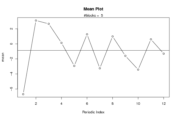
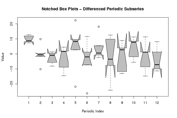
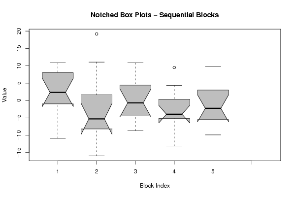
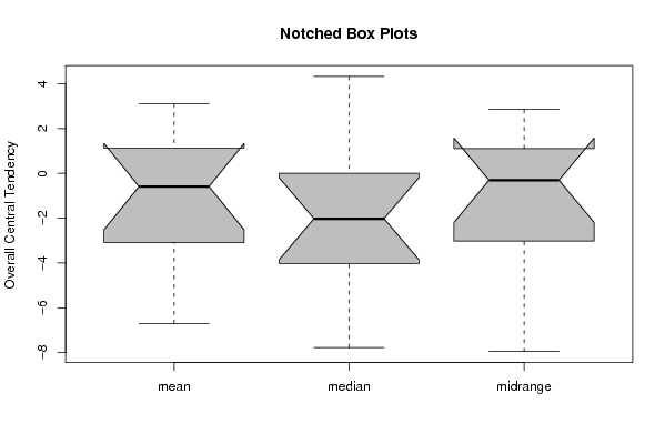
| Title produced by software | Mean Plot | ||||||||||||||||||||
| Date of computation | Thu, 03 Dec 2009 17:46:16 -0700 | ||||||||||||||||||||
| Cite this page as follows | Statistical Computations at FreeStatistics.org, Office for Research Development and Education, URL https://freestatistics.org/blog/index.php?v=date/2009/Dec/04/t12598876473r8e1qnfr70drl0.htm/, Retrieved Sun, 28 Apr 2024 00:23:23 +0000 | ||||||||||||||||||||
| Statistical Computations at FreeStatistics.org, Office for Research Development and Education, URL https://freestatistics.org/blog/index.php?pk=63159, Retrieved Sun, 28 Apr 2024 00:23:23 +0000 | |||||||||||||||||||||
| QR Codes: | |||||||||||||||||||||
|
| |||||||||||||||||||||
| Original text written by user: | |||||||||||||||||||||
| IsPrivate? | No (this computation is public) | ||||||||||||||||||||
| User-defined keywords | |||||||||||||||||||||
| Estimated Impact | 153 | ||||||||||||||||||||
Tree of Dependent Computations | |||||||||||||||||||||
| Family? (F = Feedback message, R = changed R code, M = changed R Module, P = changed Parameters, D = changed Data) | |||||||||||||||||||||
| - [Univariate Data Series] [data set] [2008-12-01 19:54:57] [b98453cac15ba1066b407e146608df68] - RMP [ARIMA Backward Selection] [] [2009-11-27 14:53:14] [b98453cac15ba1066b407e146608df68] F RM D [Mean Plot] [WS9] [2009-12-04 00:46:16] [557d56ec4b06cd0135c259898de8ce95] [Current] | |||||||||||||||||||||
| Feedback Forum | |||||||||||||||||||||
Post a new message | |||||||||||||||||||||
Dataset | |||||||||||||||||||||
| Dataseries X: | |||||||||||||||||||||
0.101412434656184 8.81202575001982 7.22218199005616 6.34522390407069 10.8649940993359 -10.8922198651649 0.734394414465646 -0.0179390706289798 9.77474289606975 -1.89838978467021 -7.43663216780881 3.93631177801305 -7.37586328597002 4.56937607566163 -5.57644511931599 -5.01498813962224 -3.15959218858348 19.1892932271942 -7.06045860990475 11.0833125612922 -13.0458821593181 -9.06290124399022 -1.28060038228237 -15.9882579614673 -7.77520617937238 -0.433574311074287 9.42649047423882 10.8410822582803 -3.69645197084187 -0.959561390175432 -2.93909670762435 -5.22988378451808 -8.70332470272302 0.20118534528325 8.63697951799477 0.0353594847692281 -8.52606038876601 4.32479728273804 3.77674215942339 -4.3395217968542 -13.1524297646555 -4.89269052015993 -3.64581392623976 -3.03944041822005 9.51943698875795 -3.59266175781745 -5.48035015252675 -4.25254907793764 -9.9008973968445 -1.75816861848705 -1.52563999886315 -7.18999545624147 -5.51845416493396 3.89790349608751 -3.35322089064957 2.13650137374166 -5.51652882241756 -2.76178813847456 8.56498835185603 9.7467700827992 | |||||||||||||||||||||
Tables (Output of Computation) | |||||||||||||||||||||
| |||||||||||||||||||||
Figures (Output of Computation) | |||||||||||||||||||||
Input Parameters & R Code | |||||||||||||||||||||
| Parameters (Session): | |||||||||||||||||||||
| par1 = FALSE ; par2 = 0.5 ; par3 = 1 ; par4 = 1 ; par5 = 12 ; par6 = 3 ; par7 = 1 ; par8 = 2 ; par9 = 1 ; | |||||||||||||||||||||
| Parameters (R input): | |||||||||||||||||||||
| par1 = 12 ; | |||||||||||||||||||||
| R code (references can be found in the software module): | |||||||||||||||||||||
par1 <- as.numeric(par1) | |||||||||||||||||||||