Free Statistics
of Irreproducible Research!
Description of Statistical Computation | |||||||||||||||||||||
|---|---|---|---|---|---|---|---|---|---|---|---|---|---|---|---|---|---|---|---|---|---|
| Author's title | |||||||||||||||||||||
| Author | *The author of this computation has been verified* | ||||||||||||||||||||
| R Software Module | rwasp_meanplot.wasp | ||||||||||||||||||||
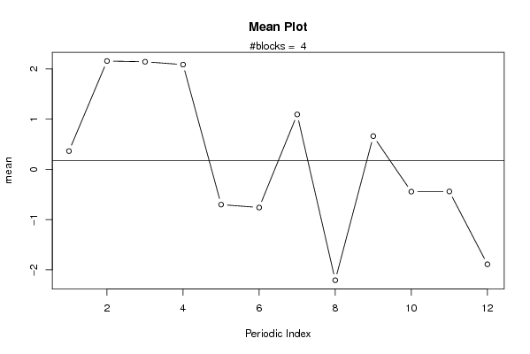
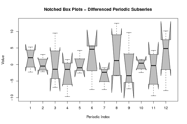
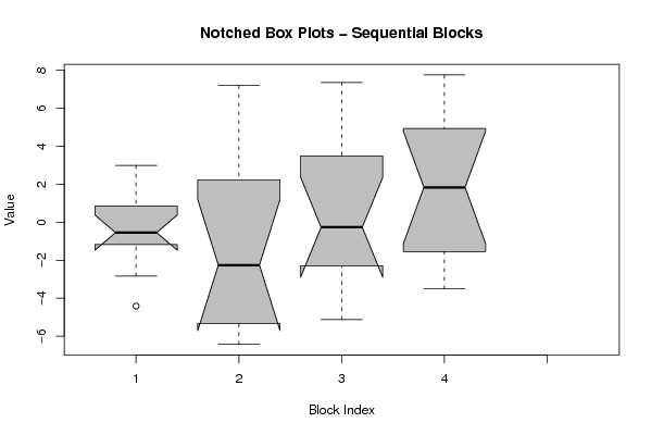
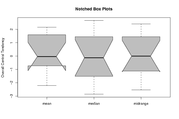
| Title produced by software | Mean Plot | ||||||||||||||||||||
| Date of computation | Fri, 04 Dec 2009 04:57:21 -0700 | ||||||||||||||||||||
| Cite this page as follows | Statistical Computations at FreeStatistics.org, Office for Research Development and Education, URL https://freestatistics.org/blog/index.php?v=date/2009/Dec/04/t1259927920giz24i88ruk4bmv.htm/, Retrieved Sat, 27 Apr 2024 17:34:29 +0000 | ||||||||||||||||||||
| Statistical Computations at FreeStatistics.org, Office for Research Development and Education, URL https://freestatistics.org/blog/index.php?pk=63333, Retrieved Sat, 27 Apr 2024 17:34:29 +0000 | |||||||||||||||||||||
| QR Codes: | |||||||||||||||||||||
|
| |||||||||||||||||||||
| Original text written by user: | |||||||||||||||||||||
| IsPrivate? | No (this computation is public) | ||||||||||||||||||||
| User-defined keywords | |||||||||||||||||||||
| Estimated Impact | 150 | ||||||||||||||||||||
Tree of Dependent Computations | |||||||||||||||||||||
| Family? (F = Feedback message, R = changed R code, M = changed R Module, P = changed Parameters, D = changed Data) | |||||||||||||||||||||
| - [Univariate Data Series] [data set] [2008-12-01 19:54:57] [b98453cac15ba1066b407e146608df68] - RMP [ARIMA Backward Selection] [] [2009-11-27 14:53:14] [b98453cac15ba1066b407e146608df68] - D [ARIMA Backward Selection] [BBWS9-Arimabackward1] [2009-12-01 20:26:03] [408e92805dcb18620260f240a7fb9d53] - RM D [Harrell-Davis Quantiles] [BBWS9-Harolddavis] [2009-12-01 20:39:11] [408e92805dcb18620260f240a7fb9d53] - RM [Mean Plot] [BBWS9-Meanplot] [2009-12-01 20:43:16] [408e92805dcb18620260f240a7fb9d53] - PD [Mean Plot] [workshop 9] [2009-12-04 11:57:21] [6c94b261890ba36343a04d1029691995] [Current] - D [Mean Plot] [workshop 9] [2009-12-08 21:17:21] [28d531aeb5ea2ff1b676cbab66947a19] | |||||||||||||||||||||
| Feedback Forum | |||||||||||||||||||||
Post a new message | |||||||||||||||||||||
Dataset | |||||||||||||||||||||
| Dataseries X: | |||||||||||||||||||||
-0.960413185401952 -0.257096857061657 -0.00305097423970006 -1.22060840651389 0.281147854452748 -0.837214034024459 2.99538578499307 2.01192824719042 -1.13142847782208 -4.41735107993375 -2.84326720390843 1.42420708592824 -6.4319528185145 -1.15134540051891 -2.31759658186013 7.19405393968334 -2.51152222562894 -5.05067246799101 0.633609505899342 -2.19833108044682 -5.61600895377663 4.06077142955234 3.81497929522652 -5.63333124192523 4.54262532082878 2.2869987279077 5.31788785818883 -1.57767876248737 -2.20767339276594 -3.03004636377187 2.4221089067681 -5.13003966404093 7.35432758766906 0.00333765818966027 -2.39180447559783 -0.536093770338058 4.30423414238618 7.75062996097202 5.5738788229018 3.94690741416824 1.63005802585319 5.87623150802847 -1.6770930063302 -3.51531169044285 2.03885369634053 -1.42127033457145 -0.340892797342981 -2.81624738305871 | |||||||||||||||||||||
Tables (Output of Computation) | |||||||||||||||||||||
| |||||||||||||||||||||
Figures (Output of Computation) | |||||||||||||||||||||
Input Parameters & R Code | |||||||||||||||||||||
| Parameters (Session): | |||||||||||||||||||||
| par1 = 12 ; | |||||||||||||||||||||
| Parameters (R input): | |||||||||||||||||||||
| par1 = 12 ; | |||||||||||||||||||||
| R code (references can be found in the software module): | |||||||||||||||||||||
par1 <- as.numeric(par1) | |||||||||||||||||||||