Repository of Reproducible Computations

Free Statistics

of Irreproducible Research!

Author's title

Author

*The author of this computation has been verified*

R Software Module

rwasp_autocorrelation.wasp

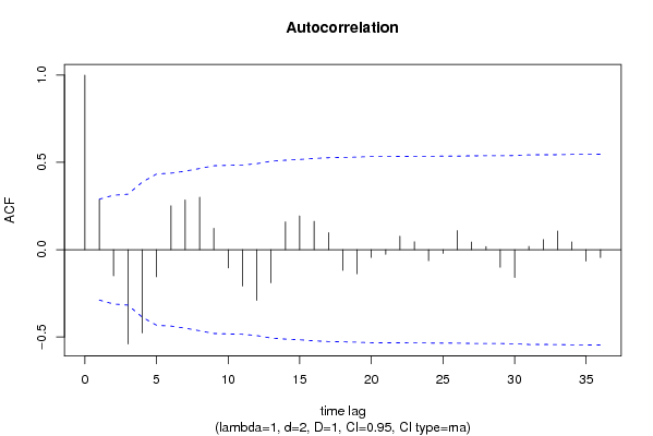
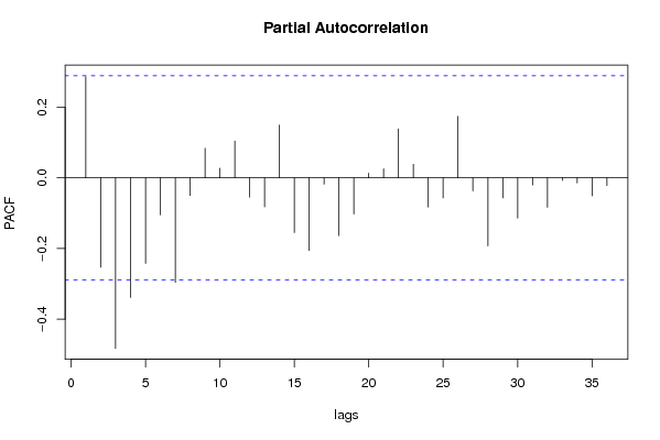
Title produced by software

(Partial) Autocorrelation Function

Date of computation

Fri, 04 Dec 2009 05:40:35 -0700

Cite this page as follows

Statistical Computations at FreeStatistics.org, Office for Research Development and Education, URL https://freestatistics.org/blog/index.php?v=date/2009/Dec/04/t125993080030bn454q7c5njjy.htm/, Retrieved Sun, 28 Apr 2024 12:19:59 +0000

Statistical Computations at FreeStatistics.org, Office for Research Development and Education, URL https://freestatistics.org/blog/index.php?pk=63432, Retrieved Sun, 28 Apr 2024 12:19:59 +0000

QR Codes:

Paste this QR Code to cite your computation.

Original text written by user:

IsPrivate?

No (this computation is public)

User-defined keywords

Estimated Impact

134

Family? (F = Feedback message, R = changed R code, M = changed R Module, P = changed Parameters, D = changed Data)

-     [Univariate Data Series] [data set] [2008-12-01 19:54:57] [b98453cac15ba1066b407e146608df68]
- RMP   [(Partial) Autocorrelation Function] [] [2009-11-27 14:46:03] [b98453cac15ba1066b407e146608df68]
-    D    [(Partial) Autocorrelation Function] [WS9-ACF] [2009-12-04 12:29:51] [a94022e7c2399c0f4d62eea578db3411]
-   P       [(Partial) Autocorrelation Function] [WS9-ACF2] [2009-12-04 12:34:59] [a94022e7c2399c0f4d62eea578db3411]
-   P           [(Partial) Autocorrelation Function] [] [2009-12-04 12:40:35] [30970b478e356ce7f8c2e9fca280b230] [Current]
-   PD            [(Partial) Autocorrelation Function] [ACF en PACF Oefen...] [2009-12-18 12:21:26] [a94022e7c2399c0f4d62eea578db3411] 
- R  D            [(Partial) Autocorrelation Function] [] [2010-12-07 09:28:30] [d7b28a0391ab3b2ddc9f9fba95a43f33] 
-    D            [(Partial) Autocorrelation Function] [] [2010-12-07 09:27:07] [fb3a7008aea9486db3846dc25434607b] 

Feedback Forum

Post a new message

Dataseries X:

Download CSV

Histogram

Boxplots

10.9
10
9.2
9.2
9.5
9.6
9.5
9.1
8.9
9
10.1
10.3
10.2
9.6
9.2
9.3
9.4
9.4
9.2
9
9
9
9.8
10
9.8
9.3
9
9
9.1
9.1
9.1
9.2
8.8
8.3
8.4
8.1
7.7
7.9
7.9
8
7.9
7.6
7.1
6.8
6.5
6.9
8.2
8.7
8.3
7.9
7.5
7.8
8.3
8.4
8.2
7.7
7.2
7.3
8.1
8.5

Summary of computational transaction
Raw Input	view raw input (R code)
Raw Output	view raw output of R engine
Computing time	1 seconds
R Server	'Gwilym Jenkins' @ 72.249.127.135

\begin{tabular}{lllllllll}
\hline
Summary of computational transaction \tabularnewline
Raw Input & view raw input (R code)  \tabularnewline
Raw Output & view raw output of R engine  \tabularnewline
Computing time & 1 seconds \tabularnewline
R Server & 'Gwilym Jenkins' @ 72.249.127.135 \tabularnewline
\hline
\end{tabular}
%Source: https://freestatistics.org/blog/index.php?pk=63432&T=0

[TABLE]
[ROW][C]Summary of computational transaction[/C][/ROW]
[ROW][C]Raw Input[/C][C]view raw input (R code) [/C][/ROW]
[ROW][C]Raw Output[/C][C]view raw output of R engine [/C][/ROW]
[ROW][C]Computing time[/C][C]1 seconds[/C][/ROW]
[ROW][C]R Server[/C][C]'Gwilym Jenkins' @ 72.249.127.135[/C][/ROW]
[/TABLE]
Source: https://freestatistics.org/blog/index.php?pk=63432&T=0

Globally Unique Identifier (entire table): ba.freestatistics.org/blog/index.php?pk=63432&T=0

As an alternative you can also use a QR Code:

The GUIDs for individual cells are displayed in the table below:

Summary of computational transaction
Raw Input	view raw input (R code)
Raw Output	view raw output of R engine
Computing time	1 seconds
R Server	'Gwilym Jenkins' @ 72.249.127.135

Autocorrelation Function
Time lag k	ACF(k)	T-STAT	P-value
1	0.286508	1.9432	0.029064
2	-0.149851	-1.0163	0.157392
3	-0.540721	-3.6673	0.000317
4	-0.47769	-3.2399	0.001112
5	-0.155691	-1.056	0.148253
6	0.251256	1.7041	0.047555
7	0.284902	1.9323	0.029747
8	0.300535	2.0383	0.023645
9	0.12261	0.8316	0.204971
10	-0.104621	-0.7096	0.240776
11	-0.208893	-1.4168	0.081642
12	-0.290497	-1.9702	0.027424
13	-0.189838	-1.2875	0.102172
14	0.159332	1.0806	0.142745
15	0.193054	1.3094	0.098458
16	0.162435	1.1017	0.138165
17	0.097011	0.658	0.256921
18	-0.11877	-0.8055	0.212326
19	-0.138628	-0.9402	0.176008
20	-0.044991	-0.3051	0.380815
21	-0.02684	-0.182	0.428178
22	0.077024	0.5224	0.301948
23	0.045337	0.3075	0.37993
24	-0.063591	-0.4313	0.334133
25	-0.021168	-0.1436	0.443233
26	0.109333	0.7415	0.23107
27	0.043223	0.2932	0.385363
28	0.018099	0.1228	0.451419
29	-0.101133	-0.6859	0.248104
30	-0.159534	-1.082	0.142443
31	0.018746	0.1271	0.449692
32	0.057734	0.3916	0.348591
33	0.106721	0.7238	0.236421
34	0.044122	0.2993	0.383049
35	-0.065569	-0.4447	0.329307
36	-0.045204	-0.3066	0.38027

\begin{tabular}{lllllllll}
\hline
Autocorrelation Function \tabularnewline
Time lag k & ACF(k) & T-STAT & P-value \tabularnewline
1 & 0.286508 & 1.9432 & 0.029064 \tabularnewline
2 & -0.149851 & -1.0163 & 0.157392 \tabularnewline
3 & -0.540721 & -3.6673 & 0.000317 \tabularnewline
4 & -0.47769 & -3.2399 & 0.001112 \tabularnewline
5 & -0.155691 & -1.056 & 0.148253 \tabularnewline
6 & 0.251256 & 1.7041 & 0.047555 \tabularnewline
7 & 0.284902 & 1.9323 & 0.029747 \tabularnewline
8 & 0.300535 & 2.0383 & 0.023645 \tabularnewline
9 & 0.12261 & 0.8316 & 0.204971 \tabularnewline
10 & -0.104621 & -0.7096 & 0.240776 \tabularnewline
11 & -0.208893 & -1.4168 & 0.081642 \tabularnewline
12 & -0.290497 & -1.9702 & 0.027424 \tabularnewline
13 & -0.189838 & -1.2875 & 0.102172 \tabularnewline
14 & 0.159332 & 1.0806 & 0.142745 \tabularnewline
15 & 0.193054 & 1.3094 & 0.098458 \tabularnewline
16 & 0.162435 & 1.1017 & 0.138165 \tabularnewline
17 & 0.097011 & 0.658 & 0.256921 \tabularnewline
18 & -0.11877 & -0.8055 & 0.212326 \tabularnewline
19 & -0.138628 & -0.9402 & 0.176008 \tabularnewline
20 & -0.044991 & -0.3051 & 0.380815 \tabularnewline
21 & -0.02684 & -0.182 & 0.428178 \tabularnewline
22 & 0.077024 & 0.5224 & 0.301948 \tabularnewline
23 & 0.045337 & 0.3075 & 0.37993 \tabularnewline
24 & -0.063591 & -0.4313 & 0.334133 \tabularnewline
25 & -0.021168 & -0.1436 & 0.443233 \tabularnewline
26 & 0.109333 & 0.7415 & 0.23107 \tabularnewline
27 & 0.043223 & 0.2932 & 0.385363 \tabularnewline
28 & 0.018099 & 0.1228 & 0.451419 \tabularnewline
29 & -0.101133 & -0.6859 & 0.248104 \tabularnewline
30 & -0.159534 & -1.082 & 0.142443 \tabularnewline
31 & 0.018746 & 0.1271 & 0.449692 \tabularnewline
32 & 0.057734 & 0.3916 & 0.348591 \tabularnewline
33 & 0.106721 & 0.7238 & 0.236421 \tabularnewline
34 & 0.044122 & 0.2993 & 0.383049 \tabularnewline
35 & -0.065569 & -0.4447 & 0.329307 \tabularnewline
36 & -0.045204 & -0.3066 & 0.38027 \tabularnewline
\hline
\end{tabular}
%Source: https://freestatistics.org/blog/index.php?pk=63432&T=1

[TABLE]
[ROW][C]Autocorrelation Function[/C][/ROW]
[ROW][C]Time lag k[/C][C]ACF(k)[/C][C]T-STAT[/C][C]P-value[/C][/ROW]
[ROW][C]1[/C][C]0.286508[/C][C]1.9432[/C][C]0.029064[/C][/ROW]
[ROW][C]2[/C][C]-0.149851[/C][C]-1.0163[/C][C]0.157392[/C][/ROW]
[ROW][C]3[/C][C]-0.540721[/C][C]-3.6673[/C][C]0.000317[/C][/ROW]
[ROW][C]4[/C][C]-0.47769[/C][C]-3.2399[/C][C]0.001112[/C][/ROW]
[ROW][C]5[/C][C]-0.155691[/C][C]-1.056[/C][C]0.148253[/C][/ROW]
[ROW][C]6[/C][C]0.251256[/C][C]1.7041[/C][C]0.047555[/C][/ROW]
[ROW][C]7[/C][C]0.284902[/C][C]1.9323[/C][C]0.029747[/C][/ROW]
[ROW][C]8[/C][C]0.300535[/C][C]2.0383[/C][C]0.023645[/C][/ROW]
[ROW][C]9[/C][C]0.12261[/C][C]0.8316[/C][C]0.204971[/C][/ROW]
[ROW][C]10[/C][C]-0.104621[/C][C]-0.7096[/C][C]0.240776[/C][/ROW]
[ROW][C]11[/C][C]-0.208893[/C][C]-1.4168[/C][C]0.081642[/C][/ROW]
[ROW][C]12[/C][C]-0.290497[/C][C]-1.9702[/C][C]0.027424[/C][/ROW]
[ROW][C]13[/C][C]-0.189838[/C][C]-1.2875[/C][C]0.102172[/C][/ROW]
[ROW][C]14[/C][C]0.159332[/C][C]1.0806[/C][C]0.142745[/C][/ROW]
[ROW][C]15[/C][C]0.193054[/C][C]1.3094[/C][C]0.098458[/C][/ROW]
[ROW][C]16[/C][C]0.162435[/C][C]1.1017[/C][C]0.138165[/C][/ROW]
[ROW][C]17[/C][C]0.097011[/C][C]0.658[/C][C]0.256921[/C][/ROW]
[ROW][C]18[/C][C]-0.11877[/C][C]-0.8055[/C][C]0.212326[/C][/ROW]
[ROW][C]19[/C][C]-0.138628[/C][C]-0.9402[/C][C]0.176008[/C][/ROW]
[ROW][C]20[/C][C]-0.044991[/C][C]-0.3051[/C][C]0.380815[/C][/ROW]
[ROW][C]21[/C][C]-0.02684[/C][C]-0.182[/C][C]0.428178[/C][/ROW]
[ROW][C]22[/C][C]0.077024[/C][C]0.5224[/C][C]0.301948[/C][/ROW]
[ROW][C]23[/C][C]0.045337[/C][C]0.3075[/C][C]0.37993[/C][/ROW]
[ROW][C]24[/C][C]-0.063591[/C][C]-0.4313[/C][C]0.334133[/C][/ROW]
[ROW][C]25[/C][C]-0.021168[/C][C]-0.1436[/C][C]0.443233[/C][/ROW]
[ROW][C]26[/C][C]0.109333[/C][C]0.7415[/C][C]0.23107[/C][/ROW]
[ROW][C]27[/C][C]0.043223[/C][C]0.2932[/C][C]0.385363[/C][/ROW]
[ROW][C]28[/C][C]0.018099[/C][C]0.1228[/C][C]0.451419[/C][/ROW]
[ROW][C]29[/C][C]-0.101133[/C][C]-0.6859[/C][C]0.248104[/C][/ROW]
[ROW][C]30[/C][C]-0.159534[/C][C]-1.082[/C][C]0.142443[/C][/ROW]
[ROW][C]31[/C][C]0.018746[/C][C]0.1271[/C][C]0.449692[/C][/ROW]
[ROW][C]32[/C][C]0.057734[/C][C]0.3916[/C][C]0.348591[/C][/ROW]
[ROW][C]33[/C][C]0.106721[/C][C]0.7238[/C][C]0.236421[/C][/ROW]
[ROW][C]34[/C][C]0.044122[/C][C]0.2993[/C][C]0.383049[/C][/ROW]
[ROW][C]35[/C][C]-0.065569[/C][C]-0.4447[/C][C]0.329307[/C][/ROW]
[ROW][C]36[/C][C]-0.045204[/C][C]-0.3066[/C][C]0.38027[/C][/ROW]
[/TABLE]
Source: https://freestatistics.org/blog/index.php?pk=63432&T=1

Globally Unique Identifier (entire table): ba.freestatistics.org/blog/index.php?pk=63432&T=1

As an alternative you can also use a QR Code:

The GUIDs for individual cells are displayed in the table below:

Autocorrelation Function
Time lag k	ACF(k)	T-STAT	P-value
1	0.286508	1.9432	0.029064
2	-0.149851	-1.0163	0.157392
3	-0.540721	-3.6673	0.000317
4	-0.47769	-3.2399	0.001112
5	-0.155691	-1.056	0.148253
6	0.251256	1.7041	0.047555
7	0.284902	1.9323	0.029747
8	0.300535	2.0383	0.023645
9	0.12261	0.8316	0.204971
10	-0.104621	-0.7096	0.240776
11	-0.208893	-1.4168	0.081642
12	-0.290497	-1.9702	0.027424
13	-0.189838	-1.2875	0.102172
14	0.159332	1.0806	0.142745
15	0.193054	1.3094	0.098458
16	0.162435	1.1017	0.138165
17	0.097011	0.658	0.256921
18	-0.11877	-0.8055	0.212326
19	-0.138628	-0.9402	0.176008
20	-0.044991	-0.3051	0.380815
21	-0.02684	-0.182	0.428178
22	0.077024	0.5224	0.301948
23	0.045337	0.3075	0.37993
24	-0.063591	-0.4313	0.334133
25	-0.021168	-0.1436	0.443233
26	0.109333	0.7415	0.23107
27	0.043223	0.2932	0.385363
28	0.018099	0.1228	0.451419
29	-0.101133	-0.6859	0.248104
30	-0.159534	-1.082	0.142443
31	0.018746	0.1271	0.449692
32	0.057734	0.3916	0.348591
33	0.106721	0.7238	0.236421
34	0.044122	0.2993	0.383049
35	-0.065569	-0.4447	0.329307
36	-0.045204	-0.3066	0.38027

Partial Autocorrelation Function
Time lag k	PACF(k)	T-STAT	P-value
1	0.286508	1.9432	0.029064
2	-0.252679	-1.7138	0.046653
3	-0.482417	-3.2719	0.001015
4	-0.338588	-2.2964	0.013128
5	-0.242112	-1.6421	0.053696
6	-0.104651	-0.7098	0.240712
7	-0.295906	-2.0069	0.025327
8	-0.049804	-0.3378	0.368531
9	0.083736	0.5679	0.286425
10	0.027404	0.1859	0.426686
11	0.104618	0.7096	0.240781
12	-0.054182	-0.3675	0.357472
13	-0.081832	-0.555	0.290787
14	0.149817	1.0161	0.157446
15	-0.154706	-1.0493	0.149769
16	-0.205522	-1.3939	0.08502
17	-0.017606	-0.1194	0.452734
18	-0.163405	-1.1083	0.136755
19	-0.102261	-0.6936	0.24572
20	0.01337	0.0907	0.46407
21	0.025903	0.1757	0.430658
22	0.138879	0.9419	0.175577
23	0.038919	0.264	0.396494
24	-0.082431	-0.5591	0.28941
25	-0.056518	-0.3833	0.351622
26	0.174362	1.1826	0.121526
27	-0.036755	-0.2493	0.402125
28	-0.192676	-1.3068	0.09889
29	-0.056598	-0.3839	0.351422
30	-0.113733	-0.7714	0.222214
31	-0.019931	-0.1352	0.446529
32	-0.083122	-0.5638	0.287826
33	-0.007397	-0.0502	0.480102
34	-0.014245	-0.0966	0.461726
35	-0.050895	-0.3452	0.365763
36	-0.021568	-0.1463	0.44217

\begin{tabular}{lllllllll}
\hline
Partial Autocorrelation Function \tabularnewline
Time lag k & PACF(k) & T-STAT & P-value \tabularnewline
1 & 0.286508 & 1.9432 & 0.029064 \tabularnewline
2 & -0.252679 & -1.7138 & 0.046653 \tabularnewline
3 & -0.482417 & -3.2719 & 0.001015 \tabularnewline
4 & -0.338588 & -2.2964 & 0.013128 \tabularnewline
5 & -0.242112 & -1.6421 & 0.053696 \tabularnewline
6 & -0.104651 & -0.7098 & 0.240712 \tabularnewline
7 & -0.295906 & -2.0069 & 0.025327 \tabularnewline
8 & -0.049804 & -0.3378 & 0.368531 \tabularnewline
9 & 0.083736 & 0.5679 & 0.286425 \tabularnewline
10 & 0.027404 & 0.1859 & 0.426686 \tabularnewline
11 & 0.104618 & 0.7096 & 0.240781 \tabularnewline
12 & -0.054182 & -0.3675 & 0.357472 \tabularnewline
13 & -0.081832 & -0.555 & 0.290787 \tabularnewline
14 & 0.149817 & 1.0161 & 0.157446 \tabularnewline
15 & -0.154706 & -1.0493 & 0.149769 \tabularnewline
16 & -0.205522 & -1.3939 & 0.08502 \tabularnewline
17 & -0.017606 & -0.1194 & 0.452734 \tabularnewline
18 & -0.163405 & -1.1083 & 0.136755 \tabularnewline
19 & -0.102261 & -0.6936 & 0.24572 \tabularnewline
20 & 0.01337 & 0.0907 & 0.46407 \tabularnewline
21 & 0.025903 & 0.1757 & 0.430658 \tabularnewline
22 & 0.138879 & 0.9419 & 0.175577 \tabularnewline
23 & 0.038919 & 0.264 & 0.396494 \tabularnewline
24 & -0.082431 & -0.5591 & 0.28941 \tabularnewline
25 & -0.056518 & -0.3833 & 0.351622 \tabularnewline
26 & 0.174362 & 1.1826 & 0.121526 \tabularnewline
27 & -0.036755 & -0.2493 & 0.402125 \tabularnewline
28 & -0.192676 & -1.3068 & 0.09889 \tabularnewline
29 & -0.056598 & -0.3839 & 0.351422 \tabularnewline
30 & -0.113733 & -0.7714 & 0.222214 \tabularnewline
31 & -0.019931 & -0.1352 & 0.446529 \tabularnewline
32 & -0.083122 & -0.5638 & 0.287826 \tabularnewline
33 & -0.007397 & -0.0502 & 0.480102 \tabularnewline
34 & -0.014245 & -0.0966 & 0.461726 \tabularnewline
35 & -0.050895 & -0.3452 & 0.365763 \tabularnewline
36 & -0.021568 & -0.1463 & 0.44217 \tabularnewline
\hline
\end{tabular}
%Source: https://freestatistics.org/blog/index.php?pk=63432&T=2

[TABLE]
[ROW][C]Partial Autocorrelation Function[/C][/ROW]
[ROW][C]Time lag k[/C][C]PACF(k)[/C][C]T-STAT[/C][C]P-value[/C][/ROW]
[ROW][C]1[/C][C]0.286508[/C][C]1.9432[/C][C]0.029064[/C][/ROW]
[ROW][C]2[/C][C]-0.252679[/C][C]-1.7138[/C][C]0.046653[/C][/ROW]
[ROW][C]3[/C][C]-0.482417[/C][C]-3.2719[/C][C]0.001015[/C][/ROW]
[ROW][C]4[/C][C]-0.338588[/C][C]-2.2964[/C][C]0.013128[/C][/ROW]
[ROW][C]5[/C][C]-0.242112[/C][C]-1.6421[/C][C]0.053696[/C][/ROW]
[ROW][C]6[/C][C]-0.104651[/C][C]-0.7098[/C][C]0.240712[/C][/ROW]
[ROW][C]7[/C][C]-0.295906[/C][C]-2.0069[/C][C]0.025327[/C][/ROW]
[ROW][C]8[/C][C]-0.049804[/C][C]-0.3378[/C][C]0.368531[/C][/ROW]
[ROW][C]9[/C][C]0.083736[/C][C]0.5679[/C][C]0.286425[/C][/ROW]
[ROW][C]10[/C][C]0.027404[/C][C]0.1859[/C][C]0.426686[/C][/ROW]
[ROW][C]11[/C][C]0.104618[/C][C]0.7096[/C][C]0.240781[/C][/ROW]
[ROW][C]12[/C][C]-0.054182[/C][C]-0.3675[/C][C]0.357472[/C][/ROW]
[ROW][C]13[/C][C]-0.081832[/C][C]-0.555[/C][C]0.290787[/C][/ROW]
[ROW][C]14[/C][C]0.149817[/C][C]1.0161[/C][C]0.157446[/C][/ROW]
[ROW][C]15[/C][C]-0.154706[/C][C]-1.0493[/C][C]0.149769[/C][/ROW]
[ROW][C]16[/C][C]-0.205522[/C][C]-1.3939[/C][C]0.08502[/C][/ROW]
[ROW][C]17[/C][C]-0.017606[/C][C]-0.1194[/C][C]0.452734[/C][/ROW]
[ROW][C]18[/C][C]-0.163405[/C][C]-1.1083[/C][C]0.136755[/C][/ROW]
[ROW][C]19[/C][C]-0.102261[/C][C]-0.6936[/C][C]0.24572[/C][/ROW]
[ROW][C]20[/C][C]0.01337[/C][C]0.0907[/C][C]0.46407[/C][/ROW]
[ROW][C]21[/C][C]0.025903[/C][C]0.1757[/C][C]0.430658[/C][/ROW]
[ROW][C]22[/C][C]0.138879[/C][C]0.9419[/C][C]0.175577[/C][/ROW]
[ROW][C]23[/C][C]0.038919[/C][C]0.264[/C][C]0.396494[/C][/ROW]
[ROW][C]24[/C][C]-0.082431[/C][C]-0.5591[/C][C]0.28941[/C][/ROW]
[ROW][C]25[/C][C]-0.056518[/C][C]-0.3833[/C][C]0.351622[/C][/ROW]
[ROW][C]26[/C][C]0.174362[/C][C]1.1826[/C][C]0.121526[/C][/ROW]
[ROW][C]27[/C][C]-0.036755[/C][C]-0.2493[/C][C]0.402125[/C][/ROW]
[ROW][C]28[/C][C]-0.192676[/C][C]-1.3068[/C][C]0.09889[/C][/ROW]
[ROW][C]29[/C][C]-0.056598[/C][C]-0.3839[/C][C]0.351422[/C][/ROW]
[ROW][C]30[/C][C]-0.113733[/C][C]-0.7714[/C][C]0.222214[/C][/ROW]
[ROW][C]31[/C][C]-0.019931[/C][C]-0.1352[/C][C]0.446529[/C][/ROW]
[ROW][C]32[/C][C]-0.083122[/C][C]-0.5638[/C][C]0.287826[/C][/ROW]
[ROW][C]33[/C][C]-0.007397[/C][C]-0.0502[/C][C]0.480102[/C][/ROW]
[ROW][C]34[/C][C]-0.014245[/C][C]-0.0966[/C][C]0.461726[/C][/ROW]
[ROW][C]35[/C][C]-0.050895[/C][C]-0.3452[/C][C]0.365763[/C][/ROW]
[ROW][C]36[/C][C]-0.021568[/C][C]-0.1463[/C][C]0.44217[/C][/ROW]
[/TABLE]
Source: https://freestatistics.org/blog/index.php?pk=63432&T=2

Globally Unique Identifier (entire table): ba.freestatistics.org/blog/index.php?pk=63432&T=2

As an alternative you can also use a QR Code:

The GUIDs for individual cells are displayed in the table below:

Partial Autocorrelation Function
Time lag k	PACF(k)	T-STAT	P-value
1	0.286508	1.9432	0.029064
2	-0.252679	-1.7138	0.046653
3	-0.482417	-3.2719	0.001015
4	-0.338588	-2.2964	0.013128
5	-0.242112	-1.6421	0.053696
6	-0.104651	-0.7098	0.240712
7	-0.295906	-2.0069	0.025327
8	-0.049804	-0.3378	0.368531
9	0.083736	0.5679	0.286425
10	0.027404	0.1859	0.426686
11	0.104618	0.7096	0.240781
12	-0.054182	-0.3675	0.357472
13	-0.081832	-0.555	0.290787
14	0.149817	1.0161	0.157446
15	-0.154706	-1.0493	0.149769
16	-0.205522	-1.3939	0.08502
17	-0.017606	-0.1194	0.452734
18	-0.163405	-1.1083	0.136755
19	-0.102261	-0.6936	0.24572
20	0.01337	0.0907	0.46407
21	0.025903	0.1757	0.430658
22	0.138879	0.9419	0.175577
23	0.038919	0.264	0.396494
24	-0.082431	-0.5591	0.28941
25	-0.056518	-0.3833	0.351622
26	0.174362	1.1826	0.121526
27	-0.036755	-0.2493	0.402125
28	-0.192676	-1.3068	0.09889
29	-0.056598	-0.3839	0.351422
30	-0.113733	-0.7714	0.222214
31	-0.019931	-0.1352	0.446529
32	-0.083122	-0.5638	0.287826
33	-0.007397	-0.0502	0.480102
34	-0.014245	-0.0966	0.461726
35	-0.050895	-0.3452	0.365763
36	-0.021568	-0.1463	0.44217

Figure 1

PNG link

Postscript link

PDF link

Figure 2

PNG link

Postscript link

PDF link

Parameters (Session):

par1 = 36 ; par2 = 1 ; par3 = 2 ; par4 = 1 ; par5 = 12 ; par6 = MA ; par7 = 0.95 ;

Parameters (R input):

par1 = 36 ; par2 = 1 ; par3 = 2 ; par4 = 1 ; par5 = 12 ; par6 = MA ; par7 = 0.95 ;

R code (references can be found in the software module):

if (par1 == 'Default') {
par1 = 10*log10(length(x))
} else {
par1 <- as.numeric(par1)
}
par2 <- as.numeric(par2)
par3 <- as.numeric(par3)
par4 <- as.numeric(par4)
par5 <- as.numeric(par5)
if (par6 == 'White Noise') par6 <- 'white' else par6 <- 'ma'
par7 <- as.numeric(par7)
if (par2 == 0) {
x <- log(x)
} else {
x <- (x ^ par2 - 1) / par2
}
if (par3 > 0) x <- diff(x,lag=1,difference=par3)
if (par4 > 0) x <- diff(x,lag=par5,difference=par4)
bitmap(file='pic1.png')
racf <- acf(x, par1, main='Autocorrelation', xlab='time lag', ylab='ACF', ci.type=par6, ci=par7, sub=paste('(lambda=',par2,', d=',par3,', D=',par4,', CI=', par7, ', CI type=',par6,')',sep=''))
dev.off()
bitmap(file='pic2.png')
rpacf <- pacf(x,par1,main='Partial Autocorrelation',xlab='lags',ylab='PACF')
dev.off()
(myacf <- c(racf$acf))
(mypacf <- c(rpacf$acf))
lengthx <- length(x)
sqrtn <- sqrt(lengthx)
load(file='createtable')
a<-table.start()
a<-table.row.start(a)
a<-table.element(a,'Autocorrelation Function',4,TRUE)
a<-table.row.end(a)
a<-table.row.start(a)
a<-table.element(a,'Time lag k',header=TRUE)
a<-table.element(a,hyperlink('basics.htm','ACF(k)','click here for more information about the Autocorrelation Function'),header=TRUE)
a<-table.element(a,'T-STAT',header=TRUE)
a<-table.element(a,'P-value',header=TRUE)
a<-table.row.end(a)
for (i in 2:(par1+1)) {
a<-table.row.start(a)
a<-table.element(a,i-1,header=TRUE)
a<-table.element(a,round(myacf[i],6))
mytstat <- myacf[i]*sqrtn
a<-table.element(a,round(mytstat,4))
a<-table.element(a,round(1-pt(abs(mytstat),lengthx),6))
a<-table.row.end(a)
}
a<-table.end(a)
table.save(a,file='mytable.tab')
a<-table.start()
a<-table.row.start(a)
a<-table.element(a,'Partial Autocorrelation Function',4,TRUE)
a<-table.row.end(a)
a<-table.row.start(a)
a<-table.element(a,'Time lag k',header=TRUE)
a<-table.element(a,hyperlink('basics.htm','PACF(k)','click here for more information about the Partial Autocorrelation Function'),header=TRUE)
a<-table.element(a,'T-STAT',header=TRUE)
a<-table.element(a,'P-value',header=TRUE)
a<-table.row.end(a)
for (i in 1:par1) {
a<-table.row.start(a)
a<-table.element(a,i,header=TRUE)
a<-table.element(a,round(mypacf[i],6))
mytstat <- mypacf[i]*sqrtn
a<-table.element(a,round(mytstat,4))
a<-table.element(a,round(1-pt(abs(mytstat),lengthx),6))
a<-table.row.end(a)
}
a<-table.end(a)
table.save(a,file='mytable1.tab')

Free Statistics

Description of Statistical Computation

Tree of Dependent Computations

Dataset

Tables (Output of Computation)

Figures (Output of Computation)

Input Parameters & R Code