Free Statistics

of Irreproducible Research!

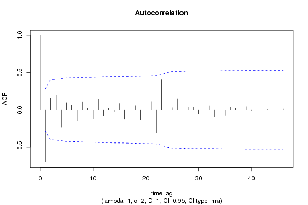
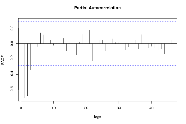
Author's title

acf - d=2, D=1, lambda = 1, - Totale industri�le productie index met basis ...

Author

*The author of this computation has been verified*

R Software Module

rwasp_autocorrelation.wasp

Title produced by software

(Partial) Autocorrelation Function

Date of computation

Fri, 04 Dec 2009 06:01:19 -0700

Cite this page as follows

Statistical Computations at FreeStatistics.org, Office for Research Development and Education, URL https://freestatistics.org/blog/index.php?v=date/2009/Dec/04/t1259932381lycuppi5apmyfpz.htm/, Retrieved Sat, 27 Apr 2024 15:21:30 +0000

Statistical Computations at FreeStatistics.org, Office for Research Development and Education, URL https://freestatistics.org/blog/index.php?pk=63466, Retrieved Sat, 27 Apr 2024 15:21:30 +0000

QR Codes:

Paste this QR Code to cite your computation.

Original text written by user:

IsPrivate?

No (this computation is public)

User-defined keywords

Estimated Impact

146

Family? (F = Feedback message, R = changed R code, M = changed R Module, P = changed Parameters, D = changed Data)

-     [Univariate Data Series] [data set] [2008-12-01 19:54:57] [b98453cac15ba1066b407e146608df68]
- RMP   [(Partial) Autocorrelation Function] [] [2009-11-27 14:46:03] [b98453cac15ba1066b407e146608df68]
-   PD    [(Partial) Autocorrelation Function] [acf - d=0, D=1, l...] [2009-12-04 00:13:44] [77c4589624c8ef9dff4002b842437335]
- R P         [(Partial) Autocorrelation Function] [acf - d=2, D=1, l...] [2009-12-04 13:01:19] [8f072ead2c7c0b3cf3fdae49bab9dd9b] [Current]
-   P           [(Partial) Autocorrelation Function] [] [2009-12-08 17:08:39] [b7349fb284cae6f1172638396d27b11f] 
- RMP           [ARIMA Backward Selection] [] [2009-12-08 17:14:36] [b7349fb284cae6f1172638396d27b11f] 
- R               [ARIMA Backward Selection] [] [2009-12-21 13:48:27] [77c4589624c8ef9dff4002b842437335] 

Feedback Forum

Post a new message

Dataseries X:

Download CSV

Histogram

Boxplots

Summary of computational transaction
Raw Input	view raw input (R code)
Raw Output	view raw output of R engine
Computing time	1 seconds
R Server	'Gwilym Jenkins' @ 72.249.127.135

\begin{tabular}{lllllllll}
\hline
Summary of computational transaction \tabularnewline
Raw Input & view raw input (R code)  \tabularnewline
Raw Output & view raw output of R engine  \tabularnewline
Computing time & 1 seconds \tabularnewline
R Server & 'Gwilym Jenkins' @ 72.249.127.135 \tabularnewline
\hline
\end{tabular}
%Source: https://freestatistics.org/blog/index.php?pk=63466&T=0

[TABLE]
[ROW][C]Summary of computational transaction[/C][/ROW]
[ROW][C]Raw Input[/C][C]view raw input (R code) [/C][/ROW]
[ROW][C]Raw Output[/C][C]view raw output of R engine [/C][/ROW]
[ROW][C]Computing time[/C][C]1 seconds[/C][/ROW]
[ROW][C]R Server[/C][C]'Gwilym Jenkins' @ 72.249.127.135[/C][/ROW]
[/TABLE]
Source: https://freestatistics.org/blog/index.php?pk=63466&T=0

Globally Unique Identifier (entire table): ba.freestatistics.org/blog/index.php?pk=63466&T=0

As an alternative you can also use a QR Code:

The GUIDs for individual cells are displayed in the table below:

Summary of computational transaction
Raw Input	view raw input (R code)
Raw Output	view raw output of R engine
Computing time	1 seconds
R Server	'Gwilym Jenkins' @ 72.249.127.135

Autocorrelation Function
Time lag k	ACF(k)	T-STAT	P-value
1	-0.704786	-4.8318	7e-06
2	0.158051	1.0835	0.142048
3	0.194163	1.3311	0.094786
4	-0.232582	-1.5945	0.058763
5	0.098205	0.6733	0.25204
6	0.066243	0.4541	0.32591
7	-0.148579	-1.0186	0.156802
8	0.103691	0.7109	0.240338
9	0.021718	0.1489	0.441138
10	-0.125175	-0.8582	0.19758
11	0.141739	0.9717	0.168083
12	-0.084685	-0.5806	0.282151
13	0.025929	0.1778	0.429838
14	-0.031348	-0.2149	0.415384
15	0.087408	0.5992	0.275945
16	-0.127565	-0.8745	0.193135
17	0.074454	0.5104	0.30607
18	0.057896	0.3969	0.346613
19	-0.139514	-0.9565	0.171867
20	0.074666	0.5119	0.305564
21	0.106022	0.7268	0.235462
22	-0.309993	-2.1252	0.019428
23	0.404062	2.7701	0.004
24	-0.287702	-1.9724	0.027233
25	0.031649	0.217	0.414584
26	0.145989	1.0008	0.161013
27	-0.137761	-0.9444	0.174888
28	0.037042	0.2539	0.400321
29	0.038415	0.2634	0.396711
30	-0.052755	-0.3617	0.359609
31	0.007211	0.0494	0.48039
32	0.056959	0.3905	0.34897
33	-0.096817	-0.6637	0.255049
34	0.10139	0.6951	0.24521
35	-0.077729	-0.5329	0.298312
36	0.034123	0.2339	0.408025
37	0.022116	0.1516	0.440067
38	-0.060225	-0.4129	0.340786
39	0.04494	0.3081	0.379686
40	-0.007841	-0.0538	0.478679
41	-0.002237	-0.0153	0.493915
42	-0.019395	-0.133	0.447395
43	0.004897	0.0336	0.486681
44	0.040824	0.2799	0.3904
45	-0.048003	-0.3291	0.371775
46	0.014891	0.1021	0.459562
47	NA	NA	NA
48	NA	NA	NA

\begin{tabular}{lllllllll}
\hline
Autocorrelation Function \tabularnewline
Time lag k & ACF(k) & T-STAT & P-value \tabularnewline
1 & -0.704786 & -4.8318 & 7e-06 \tabularnewline
2 & 0.158051 & 1.0835 & 0.142048 \tabularnewline
3 & 0.194163 & 1.3311 & 0.094786 \tabularnewline
4 & -0.232582 & -1.5945 & 0.058763 \tabularnewline
5 & 0.098205 & 0.6733 & 0.25204 \tabularnewline
6 & 0.066243 & 0.4541 & 0.32591 \tabularnewline
7 & -0.148579 & -1.0186 & 0.156802 \tabularnewline
8 & 0.103691 & 0.7109 & 0.240338 \tabularnewline
9 & 0.021718 & 0.1489 & 0.441138 \tabularnewline
10 & -0.125175 & -0.8582 & 0.19758 \tabularnewline
11 & 0.141739 & 0.9717 & 0.168083 \tabularnewline
12 & -0.084685 & -0.5806 & 0.282151 \tabularnewline
13 & 0.025929 & 0.1778 & 0.429838 \tabularnewline
14 & -0.031348 & -0.2149 & 0.415384 \tabularnewline
15 & 0.087408 & 0.5992 & 0.275945 \tabularnewline
16 & -0.127565 & -0.8745 & 0.193135 \tabularnewline
17 & 0.074454 & 0.5104 & 0.30607 \tabularnewline
18 & 0.057896 & 0.3969 & 0.346613 \tabularnewline
19 & -0.139514 & -0.9565 & 0.171867 \tabularnewline
20 & 0.074666 & 0.5119 & 0.305564 \tabularnewline
21 & 0.106022 & 0.7268 & 0.235462 \tabularnewline
22 & -0.309993 & -2.1252 & 0.019428 \tabularnewline
23 & 0.404062 & 2.7701 & 0.004 \tabularnewline
24 & -0.287702 & -1.9724 & 0.027233 \tabularnewline
25 & 0.031649 & 0.217 & 0.414584 \tabularnewline
26 & 0.145989 & 1.0008 & 0.161013 \tabularnewline
27 & -0.137761 & -0.9444 & 0.174888 \tabularnewline
28 & 0.037042 & 0.2539 & 0.400321 \tabularnewline
29 & 0.038415 & 0.2634 & 0.396711 \tabularnewline
30 & -0.052755 & -0.3617 & 0.359609 \tabularnewline
31 & 0.007211 & 0.0494 & 0.48039 \tabularnewline
32 & 0.056959 & 0.3905 & 0.34897 \tabularnewline
33 & -0.096817 & -0.6637 & 0.255049 \tabularnewline
34 & 0.10139 & 0.6951 & 0.24521 \tabularnewline
35 & -0.077729 & -0.5329 & 0.298312 \tabularnewline
36 & 0.034123 & 0.2339 & 0.408025 \tabularnewline
37 & 0.022116 & 0.1516 & 0.440067 \tabularnewline
38 & -0.060225 & -0.4129 & 0.340786 \tabularnewline
39 & 0.04494 & 0.3081 & 0.379686 \tabularnewline
40 & -0.007841 & -0.0538 & 0.478679 \tabularnewline
41 & -0.002237 & -0.0153 & 0.493915 \tabularnewline
42 & -0.019395 & -0.133 & 0.447395 \tabularnewline
43 & 0.004897 & 0.0336 & 0.486681 \tabularnewline
44 & 0.040824 & 0.2799 & 0.3904 \tabularnewline
45 & -0.048003 & -0.3291 & 0.371775 \tabularnewline
46 & 0.014891 & 0.1021 & 0.459562 \tabularnewline
47 & NA & NA & NA \tabularnewline
48 & NA & NA & NA \tabularnewline
\hline
\end{tabular}
%Source: https://freestatistics.org/blog/index.php?pk=63466&T=1

[TABLE]
[ROW][C]Autocorrelation Function[/C][/ROW]
[ROW][C]Time lag k[/C][C]ACF(k)[/C][C]T-STAT[/C][C]P-value[/C][/ROW]
[ROW][C]1[/C][C]-0.704786[/C][C]-4.8318[/C][C]7e-06[/C][/ROW]
[ROW][C]2[/C][C]0.158051[/C][C]1.0835[/C][C]0.142048[/C][/ROW]
[ROW][C]3[/C][C]0.194163[/C][C]1.3311[/C][C]0.094786[/C][/ROW]
[ROW][C]4[/C][C]-0.232582[/C][C]-1.5945[/C][C]0.058763[/C][/ROW]
[ROW][C]5[/C][C]0.098205[/C][C]0.6733[/C][C]0.25204[/C][/ROW]
[ROW][C]6[/C][C]0.066243[/C][C]0.4541[/C][C]0.32591[/C][/ROW]
[ROW][C]7[/C][C]-0.148579[/C][C]-1.0186[/C][C]0.156802[/C][/ROW]
[ROW][C]8[/C][C]0.103691[/C][C]0.7109[/C][C]0.240338[/C][/ROW]
[ROW][C]9[/C][C]0.021718[/C][C]0.1489[/C][C]0.441138[/C][/ROW]
[ROW][C]10[/C][C]-0.125175[/C][C]-0.8582[/C][C]0.19758[/C][/ROW]
[ROW][C]11[/C][C]0.141739[/C][C]0.9717[/C][C]0.168083[/C][/ROW]
[ROW][C]12[/C][C]-0.084685[/C][C]-0.5806[/C][C]0.282151[/C][/ROW]
[ROW][C]13[/C][C]0.025929[/C][C]0.1778[/C][C]0.429838[/C][/ROW]
[ROW][C]14[/C][C]-0.031348[/C][C]-0.2149[/C][C]0.415384[/C][/ROW]
[ROW][C]15[/C][C]0.087408[/C][C]0.5992[/C][C]0.275945[/C][/ROW]
[ROW][C]16[/C][C]-0.127565[/C][C]-0.8745[/C][C]0.193135[/C][/ROW]
[ROW][C]17[/C][C]0.074454[/C][C]0.5104[/C][C]0.30607[/C][/ROW]
[ROW][C]18[/C][C]0.057896[/C][C]0.3969[/C][C]0.346613[/C][/ROW]
[ROW][C]19[/C][C]-0.139514[/C][C]-0.9565[/C][C]0.171867[/C][/ROW]
[ROW][C]20[/C][C]0.074666[/C][C]0.5119[/C][C]0.305564[/C][/ROW]
[ROW][C]21[/C][C]0.106022[/C][C]0.7268[/C][C]0.235462[/C][/ROW]
[ROW][C]22[/C][C]-0.309993[/C][C]-2.1252[/C][C]0.019428[/C][/ROW]
[ROW][C]23[/C][C]0.404062[/C][C]2.7701[/C][C]0.004[/C][/ROW]
[ROW][C]24[/C][C]-0.287702[/C][C]-1.9724[/C][C]0.027233[/C][/ROW]
[ROW][C]25[/C][C]0.031649[/C][C]0.217[/C][C]0.414584[/C][/ROW]
[ROW][C]26[/C][C]0.145989[/C][C]1.0008[/C][C]0.161013[/C][/ROW]
[ROW][C]27[/C][C]-0.137761[/C][C]-0.9444[/C][C]0.174888[/C][/ROW]
[ROW][C]28[/C][C]0.037042[/C][C]0.2539[/C][C]0.400321[/C][/ROW]
[ROW][C]29[/C][C]0.038415[/C][C]0.2634[/C][C]0.396711[/C][/ROW]
[ROW][C]30[/C][C]-0.052755[/C][C]-0.3617[/C][C]0.359609[/C][/ROW]
[ROW][C]31[/C][C]0.007211[/C][C]0.0494[/C][C]0.48039[/C][/ROW]
[ROW][C]32[/C][C]0.056959[/C][C]0.3905[/C][C]0.34897[/C][/ROW]
[ROW][C]33[/C][C]-0.096817[/C][C]-0.6637[/C][C]0.255049[/C][/ROW]
[ROW][C]34[/C][C]0.10139[/C][C]0.6951[/C][C]0.24521[/C][/ROW]
[ROW][C]35[/C][C]-0.077729[/C][C]-0.5329[/C][C]0.298312[/C][/ROW]
[ROW][C]36[/C][C]0.034123[/C][C]0.2339[/C][C]0.408025[/C][/ROW]
[ROW][C]37[/C][C]0.022116[/C][C]0.1516[/C][C]0.440067[/C][/ROW]
[ROW][C]38[/C][C]-0.060225[/C][C]-0.4129[/C][C]0.340786[/C][/ROW]
[ROW][C]39[/C][C]0.04494[/C][C]0.3081[/C][C]0.379686[/C][/ROW]
[ROW][C]40[/C][C]-0.007841[/C][C]-0.0538[/C][C]0.478679[/C][/ROW]
[ROW][C]41[/C][C]-0.002237[/C][C]-0.0153[/C][C]0.493915[/C][/ROW]
[ROW][C]42[/C][C]-0.019395[/C][C]-0.133[/C][C]0.447395[/C][/ROW]
[ROW][C]43[/C][C]0.004897[/C][C]0.0336[/C][C]0.486681[/C][/ROW]
[ROW][C]44[/C][C]0.040824[/C][C]0.2799[/C][C]0.3904[/C][/ROW]
[ROW][C]45[/C][C]-0.048003[/C][C]-0.3291[/C][C]0.371775[/C][/ROW]
[ROW][C]46[/C][C]0.014891[/C][C]0.1021[/C][C]0.459562[/C][/ROW]
[ROW][C]47[/C][C]NA[/C][C]NA[/C][C]NA[/C][/ROW]
[ROW][C]48[/C][C]NA[/C][C]NA[/C][C]NA[/C][/ROW]
[/TABLE]
Source: https://freestatistics.org/blog/index.php?pk=63466&T=1

Globally Unique Identifier (entire table): ba.freestatistics.org/blog/index.php?pk=63466&T=1

As an alternative you can also use a QR Code:

The GUIDs for individual cells are displayed in the table below:

Autocorrelation Function
Time lag k	ACF(k)	T-STAT	P-value
1	-0.704786	-4.8318	7e-06
2	0.158051	1.0835	0.142048
3	0.194163	1.3311	0.094786
4	-0.232582	-1.5945	0.058763
5	0.098205	0.6733	0.25204
6	0.066243	0.4541	0.32591
7	-0.148579	-1.0186	0.156802
8	0.103691	0.7109	0.240338
9	0.021718	0.1489	0.441138
10	-0.125175	-0.8582	0.19758
11	0.141739	0.9717	0.168083
12	-0.084685	-0.5806	0.282151
13	0.025929	0.1778	0.429838
14	-0.031348	-0.2149	0.415384
15	0.087408	0.5992	0.275945
16	-0.127565	-0.8745	0.193135
17	0.074454	0.5104	0.30607
18	0.057896	0.3969	0.346613
19	-0.139514	-0.9565	0.171867
20	0.074666	0.5119	0.305564
21	0.106022	0.7268	0.235462
22	-0.309993	-2.1252	0.019428
23	0.404062	2.7701	0.004
24	-0.287702	-1.9724	0.027233
25	0.031649	0.217	0.414584
26	0.145989	1.0008	0.161013
27	-0.137761	-0.9444	0.174888
28	0.037042	0.2539	0.400321
29	0.038415	0.2634	0.396711
30	-0.052755	-0.3617	0.359609
31	0.007211	0.0494	0.48039
32	0.056959	0.3905	0.34897
33	-0.096817	-0.6637	0.255049
34	0.10139	0.6951	0.24521
35	-0.077729	-0.5329	0.298312
36	0.034123	0.2339	0.408025
37	0.022116	0.1516	0.440067
38	-0.060225	-0.4129	0.340786
39	0.04494	0.3081	0.379686
40	-0.007841	-0.0538	0.478679
41	-0.002237	-0.0153	0.493915
42	-0.019395	-0.133	0.447395
43	0.004897	0.0336	0.486681
44	0.040824	0.2799	0.3904
45	-0.048003	-0.3291	0.371775
46	0.014891	0.1021	0.459562
47	NA	NA	NA
48	NA	NA	NA

Partial Autocorrelation Function
Time lag k	PACF(k)	T-STAT	P-value
1	-0.704786	-4.8318	7e-06
2	-0.672935	-4.6134	1.5e-05
3	-0.340485	-2.3343	0.011954
4	-0.12046	-0.8258	0.206535
5	-0.03915	-0.2684	0.394784
6	0.13778	0.9446	0.174854
7	0.113654	0.7792	0.219891
8	-0.003687	-0.0253	0.48997
9	0.047935	0.3286	0.37195
10	-0.022855	-0.1567	0.438081
11	0.002088	0.0143	0.49432
12	-0.021946	-0.1505	0.440526
13	0.067047	0.4597	0.323943
14	-0.092551	-0.6345	0.264416
15	0.010977	0.0753	0.470166
16	-0.027083	-0.1857	0.426751
17	-0.147928	-1.0141	0.157853
18	0.018512	0.1269	0.449776
19	0.116583	0.7993	0.214083
20	-0.042996	-0.2948	0.384737
21	0.175548	1.2035	0.117405
22	-0.225674	-1.5471	0.064268
23	-0.024007	-0.1646	0.434989
24	0.04278	0.2933	0.385298
25	0.04695	0.3219	0.374488
26	-0.094991	-0.6512	0.259037
27	-0.038413	-0.2633	0.396718
28	0.061263	0.42	0.3382
29	0.012543	0.086	0.465918
30	0.012632	0.0866	0.465678
31	-0.027505	-0.1886	0.425623
32	-0.08521	-0.5842	0.280949
33	-0.04381	-0.3003	0.382618
34	0.0417	0.2859	0.388112
35	0.042198	0.2893	0.386815
36	-0.066206	-0.4539	0.325999
37	0.114944	0.788	0.217321
38	-0.00794	-0.0544	0.478409
39	-0.05591	-0.3833	0.351613
40	-0.035631	-0.2443	0.404042
41	-0.060269	-0.4132	0.340676
42	-0.077868	-0.5338	0.297985
43	-0.068861	-0.4721	0.319526
44	-0.132676	-0.9096	0.183843
45	0.068159	0.4673	0.32123
46	0.043371	0.2973	0.383759
47	NA	NA	NA
48	NA	NA	NA

\begin{tabular}{lllllllll}
\hline
Partial Autocorrelation Function \tabularnewline
Time lag k & PACF(k) & T-STAT & P-value \tabularnewline
1 & -0.704786 & -4.8318 & 7e-06 \tabularnewline
2 & -0.672935 & -4.6134 & 1.5e-05 \tabularnewline
3 & -0.340485 & -2.3343 & 0.011954 \tabularnewline
4 & -0.12046 & -0.8258 & 0.206535 \tabularnewline
5 & -0.03915 & -0.2684 & 0.394784 \tabularnewline
6 & 0.13778 & 0.9446 & 0.174854 \tabularnewline
7 & 0.113654 & 0.7792 & 0.219891 \tabularnewline
8 & -0.003687 & -0.0253 & 0.48997 \tabularnewline
9 & 0.047935 & 0.3286 & 0.37195 \tabularnewline
10 & -0.022855 & -0.1567 & 0.438081 \tabularnewline
11 & 0.002088 & 0.0143 & 0.49432 \tabularnewline
12 & -0.021946 & -0.1505 & 0.440526 \tabularnewline
13 & 0.067047 & 0.4597 & 0.323943 \tabularnewline
14 & -0.092551 & -0.6345 & 0.264416 \tabularnewline
15 & 0.010977 & 0.0753 & 0.470166 \tabularnewline
16 & -0.027083 & -0.1857 & 0.426751 \tabularnewline
17 & -0.147928 & -1.0141 & 0.157853 \tabularnewline
18 & 0.018512 & 0.1269 & 0.449776 \tabularnewline
19 & 0.116583 & 0.7993 & 0.214083 \tabularnewline
20 & -0.042996 & -0.2948 & 0.384737 \tabularnewline
21 & 0.175548 & 1.2035 & 0.117405 \tabularnewline
22 & -0.225674 & -1.5471 & 0.064268 \tabularnewline
23 & -0.024007 & -0.1646 & 0.434989 \tabularnewline
24 & 0.04278 & 0.2933 & 0.385298 \tabularnewline
25 & 0.04695 & 0.3219 & 0.374488 \tabularnewline
26 & -0.094991 & -0.6512 & 0.259037 \tabularnewline
27 & -0.038413 & -0.2633 & 0.396718 \tabularnewline
28 & 0.061263 & 0.42 & 0.3382 \tabularnewline
29 & 0.012543 & 0.086 & 0.465918 \tabularnewline
30 & 0.012632 & 0.0866 & 0.465678 \tabularnewline
31 & -0.027505 & -0.1886 & 0.425623 \tabularnewline
32 & -0.08521 & -0.5842 & 0.280949 \tabularnewline
33 & -0.04381 & -0.3003 & 0.382618 \tabularnewline
34 & 0.0417 & 0.2859 & 0.388112 \tabularnewline
35 & 0.042198 & 0.2893 & 0.386815 \tabularnewline
36 & -0.066206 & -0.4539 & 0.325999 \tabularnewline
37 & 0.114944 & 0.788 & 0.217321 \tabularnewline
38 & -0.00794 & -0.0544 & 0.478409 \tabularnewline
39 & -0.05591 & -0.3833 & 0.351613 \tabularnewline
40 & -0.035631 & -0.2443 & 0.404042 \tabularnewline
41 & -0.060269 & -0.4132 & 0.340676 \tabularnewline
42 & -0.077868 & -0.5338 & 0.297985 \tabularnewline
43 & -0.068861 & -0.4721 & 0.319526 \tabularnewline
44 & -0.132676 & -0.9096 & 0.183843 \tabularnewline
45 & 0.068159 & 0.4673 & 0.32123 \tabularnewline
46 & 0.043371 & 0.2973 & 0.383759 \tabularnewline
47 & NA & NA & NA \tabularnewline
48 & NA & NA & NA \tabularnewline
\hline
\end{tabular}
%Source: https://freestatistics.org/blog/index.php?pk=63466&T=2

[TABLE]
[ROW][C]Partial Autocorrelation Function[/C][/ROW]
[ROW][C]Time lag k[/C][C]PACF(k)[/C][C]T-STAT[/C][C]P-value[/C][/ROW]
[ROW][C]1[/C][C]-0.704786[/C][C]-4.8318[/C][C]7e-06[/C][/ROW]
[ROW][C]2[/C][C]-0.672935[/C][C]-4.6134[/C][C]1.5e-05[/C][/ROW]
[ROW][C]3[/C][C]-0.340485[/C][C]-2.3343[/C][C]0.011954[/C][/ROW]
[ROW][C]4[/C][C]-0.12046[/C][C]-0.8258[/C][C]0.206535[/C][/ROW]
[ROW][C]5[/C][C]-0.03915[/C][C]-0.2684[/C][C]0.394784[/C][/ROW]
[ROW][C]6[/C][C]0.13778[/C][C]0.9446[/C][C]0.174854[/C][/ROW]
[ROW][C]7[/C][C]0.113654[/C][C]0.7792[/C][C]0.219891[/C][/ROW]
[ROW][C]8[/C][C]-0.003687[/C][C]-0.0253[/C][C]0.48997[/C][/ROW]
[ROW][C]9[/C][C]0.047935[/C][C]0.3286[/C][C]0.37195[/C][/ROW]
[ROW][C]10[/C][C]-0.022855[/C][C]-0.1567[/C][C]0.438081[/C][/ROW]
[ROW][C]11[/C][C]0.002088[/C][C]0.0143[/C][C]0.49432[/C][/ROW]
[ROW][C]12[/C][C]-0.021946[/C][C]-0.1505[/C][C]0.440526[/C][/ROW]
[ROW][C]13[/C][C]0.067047[/C][C]0.4597[/C][C]0.323943[/C][/ROW]
[ROW][C]14[/C][C]-0.092551[/C][C]-0.6345[/C][C]0.264416[/C][/ROW]
[ROW][C]15[/C][C]0.010977[/C][C]0.0753[/C][C]0.470166[/C][/ROW]
[ROW][C]16[/C][C]-0.027083[/C][C]-0.1857[/C][C]0.426751[/C][/ROW]
[ROW][C]17[/C][C]-0.147928[/C][C]-1.0141[/C][C]0.157853[/C][/ROW]
[ROW][C]18[/C][C]0.018512[/C][C]0.1269[/C][C]0.449776[/C][/ROW]
[ROW][C]19[/C][C]0.116583[/C][C]0.7993[/C][C]0.214083[/C][/ROW]
[ROW][C]20[/C][C]-0.042996[/C][C]-0.2948[/C][C]0.384737[/C][/ROW]
[ROW][C]21[/C][C]0.175548[/C][C]1.2035[/C][C]0.117405[/C][/ROW]
[ROW][C]22[/C][C]-0.225674[/C][C]-1.5471[/C][C]0.064268[/C][/ROW]
[ROW][C]23[/C][C]-0.024007[/C][C]-0.1646[/C][C]0.434989[/C][/ROW]
[ROW][C]24[/C][C]0.04278[/C][C]0.2933[/C][C]0.385298[/C][/ROW]
[ROW][C]25[/C][C]0.04695[/C][C]0.3219[/C][C]0.374488[/C][/ROW]
[ROW][C]26[/C][C]-0.094991[/C][C]-0.6512[/C][C]0.259037[/C][/ROW]
[ROW][C]27[/C][C]-0.038413[/C][C]-0.2633[/C][C]0.396718[/C][/ROW]
[ROW][C]28[/C][C]0.061263[/C][C]0.42[/C][C]0.3382[/C][/ROW]
[ROW][C]29[/C][C]0.012543[/C][C]0.086[/C][C]0.465918[/C][/ROW]
[ROW][C]30[/C][C]0.012632[/C][C]0.0866[/C][C]0.465678[/C][/ROW]
[ROW][C]31[/C][C]-0.027505[/C][C]-0.1886[/C][C]0.425623[/C][/ROW]
[ROW][C]32[/C][C]-0.08521[/C][C]-0.5842[/C][C]0.280949[/C][/ROW]
[ROW][C]33[/C][C]-0.04381[/C][C]-0.3003[/C][C]0.382618[/C][/ROW]
[ROW][C]34[/C][C]0.0417[/C][C]0.2859[/C][C]0.388112[/C][/ROW]
[ROW][C]35[/C][C]0.042198[/C][C]0.2893[/C][C]0.386815[/C][/ROW]
[ROW][C]36[/C][C]-0.066206[/C][C]-0.4539[/C][C]0.325999[/C][/ROW]
[ROW][C]37[/C][C]0.114944[/C][C]0.788[/C][C]0.217321[/C][/ROW]
[ROW][C]38[/C][C]-0.00794[/C][C]-0.0544[/C][C]0.478409[/C][/ROW]
[ROW][C]39[/C][C]-0.05591[/C][C]-0.3833[/C][C]0.351613[/C][/ROW]
[ROW][C]40[/C][C]-0.035631[/C][C]-0.2443[/C][C]0.404042[/C][/ROW]
[ROW][C]41[/C][C]-0.060269[/C][C]-0.4132[/C][C]0.340676[/C][/ROW]
[ROW][C]42[/C][C]-0.077868[/C][C]-0.5338[/C][C]0.297985[/C][/ROW]
[ROW][C]43[/C][C]-0.068861[/C][C]-0.4721[/C][C]0.319526[/C][/ROW]
[ROW][C]44[/C][C]-0.132676[/C][C]-0.9096[/C][C]0.183843[/C][/ROW]
[ROW][C]45[/C][C]0.068159[/C][C]0.4673[/C][C]0.32123[/C][/ROW]
[ROW][C]46[/C][C]0.043371[/C][C]0.2973[/C][C]0.383759[/C][/ROW]
[ROW][C]47[/C][C]NA[/C][C]NA[/C][C]NA[/C][/ROW]
[ROW][C]48[/C][C]NA[/C][C]NA[/C][C]NA[/C][/ROW]
[/TABLE]
Source: https://freestatistics.org/blog/index.php?pk=63466&T=2

Globally Unique Identifier (entire table): ba.freestatistics.org/blog/index.php?pk=63466&T=2

As an alternative you can also use a QR Code:

The GUIDs for individual cells are displayed in the table below:

Partial Autocorrelation Function
Time lag k	PACF(k)	T-STAT	P-value
1	-0.704786	-4.8318	7e-06
2	-0.672935	-4.6134	1.5e-05
3	-0.340485	-2.3343	0.011954
4	-0.12046	-0.8258	0.206535
5	-0.03915	-0.2684	0.394784
6	0.13778	0.9446	0.174854
7	0.113654	0.7792	0.219891
8	-0.003687	-0.0253	0.48997
9	0.047935	0.3286	0.37195
10	-0.022855	-0.1567	0.438081
11	0.002088	0.0143	0.49432
12	-0.021946	-0.1505	0.440526
13	0.067047	0.4597	0.323943
14	-0.092551	-0.6345	0.264416
15	0.010977	0.0753	0.470166
16	-0.027083	-0.1857	0.426751
17	-0.147928	-1.0141	0.157853
18	0.018512	0.1269	0.449776
19	0.116583	0.7993	0.214083
20	-0.042996	-0.2948	0.384737
21	0.175548	1.2035	0.117405
22	-0.225674	-1.5471	0.064268
23	-0.024007	-0.1646	0.434989
24	0.04278	0.2933	0.385298
25	0.04695	0.3219	0.374488
26	-0.094991	-0.6512	0.259037
27	-0.038413	-0.2633	0.396718
28	0.061263	0.42	0.3382
29	0.012543	0.086	0.465918
30	0.012632	0.0866	0.465678
31	-0.027505	-0.1886	0.425623
32	-0.08521	-0.5842	0.280949
33	-0.04381	-0.3003	0.382618
34	0.0417	0.2859	0.388112
35	0.042198	0.2893	0.386815
36	-0.066206	-0.4539	0.325999
37	0.114944	0.788	0.217321
38	-0.00794	-0.0544	0.478409
39	-0.05591	-0.3833	0.351613
40	-0.035631	-0.2443	0.404042
41	-0.060269	-0.4132	0.340676
42	-0.077868	-0.5338	0.297985
43	-0.068861	-0.4721	0.319526
44	-0.132676	-0.9096	0.183843
45	0.068159	0.4673	0.32123
46	0.043371	0.2973	0.383759
47	NA	NA	NA
48	NA	NA	NA

Figure 1

PNG link

Postscript link

PDF link

Figure 2

PNG link

Postscript link

PDF link

Parameters (Session):

par1 = 48 ; par2 = 1 ; par3 = 2 ; par4 = 1 ; par5 = 12 ; par6 = MA ; par7 = 0.95 ;

Parameters (R input):

par1 = 48 ; par2 = 1 ; par3 = 2 ; par4 = 1 ; par5 = 12 ; par6 = MA ; par7 = 0.95 ;

R code (references can be found in the software module):

if (par1 == 'Default') {
par1 = 10*log10(length(x))
} else {
par1 <- as.numeric(par1)
}
par2 <- as.numeric(par2)
par3 <- as.numeric(par3)
par4 <- as.numeric(par4)
par5 <- as.numeric(par5)
if (par6 == 'White Noise') par6 <- 'white' else par6 <- 'ma'
par7 <- as.numeric(par7)
if (par2 == 0) {
x <- log(x)
} else {
x <- (x ^ par2 - 1) / par2
}
if (par3 > 0) x <- diff(x,lag=1,difference=par3)
if (par4 > 0) x <- diff(x,lag=par5,difference=par4)
bitmap(file='pic1.png')
racf <- acf(x, par1, main='Autocorrelation', xlab='time lag', ylab='ACF', ci.type=par6, ci=par7, sub=paste('(lambda=',par2,', d=',par3,', D=',par4,', CI=', par7, ', CI type=',par6,')',sep=''))
dev.off()
bitmap(file='pic2.png')
rpacf <- pacf(x,par1,main='Partial Autocorrelation',xlab='lags',ylab='PACF')
dev.off()
(myacf <- c(racf$acf))
(mypacf <- c(rpacf$acf))
lengthx <- length(x)
sqrtn <- sqrt(lengthx)
load(file='createtable')
a<-table.start()
a<-table.row.start(a)
a<-table.element(a,'Autocorrelation Function',4,TRUE)
a<-table.row.end(a)
a<-table.row.start(a)
a<-table.element(a,'Time lag k',header=TRUE)
a<-table.element(a,hyperlink('basics.htm','ACF(k)','click here for more information about the Autocorrelation Function'),header=TRUE)
a<-table.element(a,'T-STAT',header=TRUE)
a<-table.element(a,'P-value',header=TRUE)
a<-table.row.end(a)
for (i in 2:(par1+1)) {
a<-table.row.start(a)
a<-table.element(a,i-1,header=TRUE)
a<-table.element(a,round(myacf[i],6))
mytstat <- myacf[i]*sqrtn
a<-table.element(a,round(mytstat,4))
a<-table.element(a,round(1-pt(abs(mytstat),lengthx),6))
a<-table.row.end(a)
}
a<-table.end(a)
table.save(a,file='mytable.tab')
a<-table.start()
a<-table.row.start(a)
a<-table.element(a,'Partial Autocorrelation Function',4,TRUE)
a<-table.row.end(a)
a<-table.row.start(a)
a<-table.element(a,'Time lag k',header=TRUE)
a<-table.element(a,hyperlink('basics.htm','PACF(k)','click here for more information about the Partial Autocorrelation Function'),header=TRUE)
a<-table.element(a,'T-STAT',header=TRUE)
a<-table.element(a,'P-value',header=TRUE)
a<-table.row.end(a)
for (i in 1:par1) {
a<-table.row.start(a)
a<-table.element(a,i,header=TRUE)
a<-table.element(a,round(mypacf[i],6))
mytstat <- mypacf[i]*sqrtn
a<-table.element(a,round(mytstat,4))
a<-table.element(a,round(1-pt(abs(mytstat),lengthx),6))
a<-table.row.end(a)
}
a<-table.end(a)
table.save(a,file='mytable1.tab')

Free Statistics

Description of Statistical Computation

acf - d=2, D=1, lambda = 1, - Totale industri�le productie index met basis ...

Tree of Dependent Computations

Dataset

Tables (Output of Computation)

Figures (Output of Computation)

Input Parameters & R Code