Free Statistics
of Irreproducible Research!
Description of Statistical Computation | |||||||||||||||||||||
|---|---|---|---|---|---|---|---|---|---|---|---|---|---|---|---|---|---|---|---|---|---|
| Author's title | |||||||||||||||||||||
| Author | *The author of this computation has been verified* | ||||||||||||||||||||
| R Software Module | rwasp_meanplot.wasp | ||||||||||||||||||||
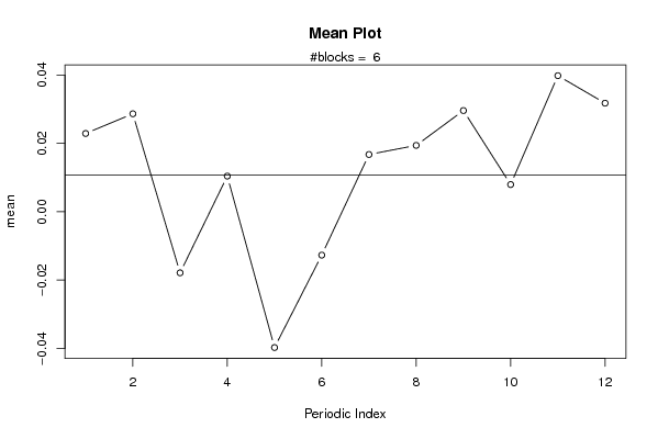
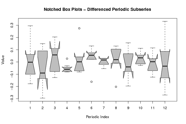
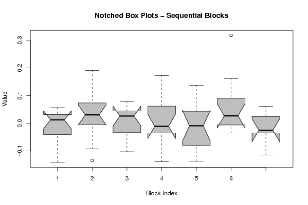
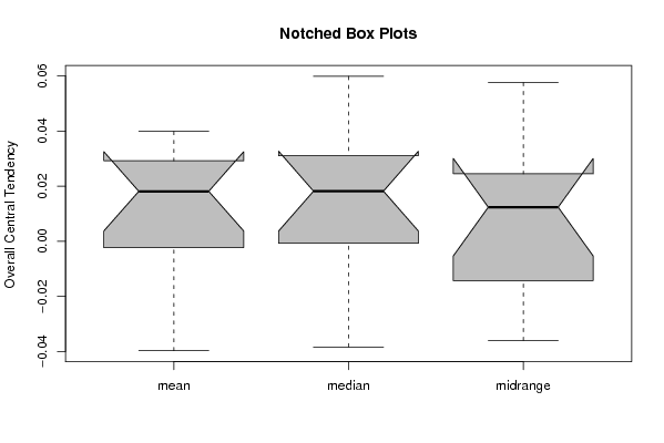
| Title produced by software | Mean Plot | ||||||||||||||||||||
| Date of computation | Fri, 04 Dec 2009 06:51:03 -0700 | ||||||||||||||||||||
| Cite this page as follows | Statistical Computations at FreeStatistics.org, Office for Research Development and Education, URL https://freestatistics.org/blog/index.php?v=date/2009/Dec/04/t1259934729asecoebi1qg71uj.htm/, Retrieved Sun, 28 Apr 2024 00:53:56 +0000 | ||||||||||||||||||||
| Statistical Computations at FreeStatistics.org, Office for Research Development and Education, URL https://freestatistics.org/blog/index.php?pk=63519, Retrieved Sun, 28 Apr 2024 00:53:56 +0000 | |||||||||||||||||||||
| QR Codes: | |||||||||||||||||||||
|
| |||||||||||||||||||||
| Original text written by user: | |||||||||||||||||||||
| IsPrivate? | No (this computation is public) | ||||||||||||||||||||
| User-defined keywords | |||||||||||||||||||||
| Estimated Impact | 109 | ||||||||||||||||||||
Tree of Dependent Computations | |||||||||||||||||||||
| Family? (F = Feedback message, R = changed R code, M = changed R Module, P = changed Parameters, D = changed Data) | |||||||||||||||||||||
| - [Univariate Data Series] [data set] [2008-12-01 19:54:57] [b98453cac15ba1066b407e146608df68] - RMP [ARIMA Backward Selection] [] [2009-11-27 14:53:14] [b98453cac15ba1066b407e146608df68] - PD [ARIMA Backward Selection] [WS9 Estimation of...] [2009-12-04 13:09:16] [8733f8ed033058987ec00f5e71b74854] - RMPD [Mean Plot] [WS9 Residu's] [2009-12-04 13:51:03] [c6e373ff11c42d4585d53e9e88ed5606] [Current] - RMP [Harrell-Davis Quantiles] [WS9 Betrouwbaarhe...] [2009-12-04 13:53:13] [8733f8ed033058987ec00f5e71b74854] - P [Harrell-Davis Quantiles] [WS9 Betrouwbaarhe...] [2009-12-04 13:55:49] [8733f8ed033058987ec00f5e71b74854] | |||||||||||||||||||||
| Feedback Forum | |||||||||||||||||||||
Post a new message | |||||||||||||||||||||
Dataset | |||||||||||||||||||||
| Dataseries X: | |||||||||||||||||||||
0.0180678527088341 0.0562901166564763 -0.0383920228971653 0.0197362615228291 -0.0349783616211472 0.0068518670200992 0.0280842746777466 0.0446752709325745 0.0346027844881839 -0.04235896700803 -0.0704530877146328 -0.141169759207391 0.190464885503065 0.0160178050891860 0.136736106377406 0.00968031609540383 -0.0209143775407505 -0.0925769658093795 0.0384619588840446 0.0682195700863305 -0.134498105554547 0.0218255727200960 0.0776457687368569 0.0689225629397706 0.0740965027033676 -0.103338356927779 -0.0429672132927176 0.0365409556880891 -0.0414354395090189 -0.012330339132303 0.0286531468201482 -0.0263319233764757 0.0785732307259898 0.0237994722126526 0.0377483003142014 0.0507363385159117 -0.0223289969571086 -0.0483741687167987 -0.138702439764697 0.0658943416950095 -0.015257998756574 -0.0966648642708767 -0.021423000325382 -0.00651105347738536 0.00512035105957504 0.073029300952841 0.0573348071614868 0.172161649472528 -0.0969619108653857 -0.0984926589389618 0.0508824323815179 -0.0623193761665625 -0.137439210181595 0.13754570197851 -0.0237979817564337 0.00561691044717635 0.0328043530195327 0.00654130655901269 0.0601321062076455 -0.0639295914075303 0.0224173380303157 0.317941659607052 0.0225647602888595 -0.0206822092677761 0.00654057567239308 -0.0190310812241401 0.0506293024636681 0.0309034012148992 0.161159786003573 -0.0350860450190002 0.0766629141540984 0.104018416656661 -0.0253219589883051 0.0607550354735824 -0.115326979930159 0.0242361757084084 -0.0348254913157667 | |||||||||||||||||||||
Tables (Output of Computation) | |||||||||||||||||||||
| |||||||||||||||||||||
Figures (Output of Computation) | |||||||||||||||||||||
Input Parameters & R Code | |||||||||||||||||||||
| Parameters (Session): | |||||||||||||||||||||
| par1 = 12 ; | |||||||||||||||||||||
| Parameters (R input): | |||||||||||||||||||||
| par1 = 12 ; | |||||||||||||||||||||
| R code (references can be found in the software module): | |||||||||||||||||||||
par1 <- as.numeric(par1) | |||||||||||||||||||||