Repository of Reproducible Computations

Free Statistics

of Irreproducible Research!

Author's title

Author

*The author of this computation has been verified*

R Software Module

rwasp_exponentialsmoothing.wasp

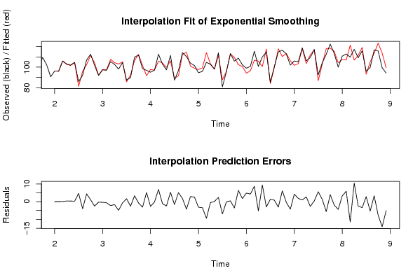
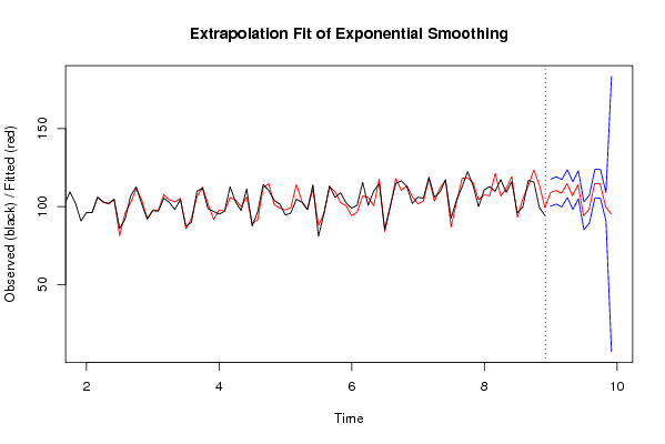
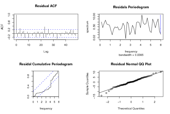
Title produced by software

Exponential Smoothing

Date of computation

Fri, 04 Dec 2009 07:35:40 -0700

Cite this page as follows

Statistical Computations at FreeStatistics.org, Office for Research Development and Education, URL https://freestatistics.org/blog/index.php?v=date/2009/Dec/04/t1259937448y8hw4ox9r82rnwr.htm/, Retrieved Sat, 27 Apr 2024 16:17:13 +0000

Statistical Computations at FreeStatistics.org, Office for Research Development and Education, URL https://freestatistics.org/blog/index.php?pk=63623, Retrieved Sat, 27 Apr 2024 16:17:13 +0000

QR Codes:

Paste this QR Code to cite your computation.

Original text written by user:

IsPrivate?

No (this computation is public)

User-defined keywords

Estimated Impact

106

Family? (F = Feedback message, R = changed R code, M = changed R Module, P = changed Parameters, D = changed Data)

-     [Univariate Data Series] [data set] [2008-12-01 19:54:57] [b98453cac15ba1066b407e146608df68]
- RMP   [Exponential Smoothing] [] [2009-11-27 15:04:36] [b98453cac15ba1066b407e146608df68]
-    D      [Exponential Smoothing] [WS 9 Exponential ...] [2009-12-04 14:35:40] [eba9f01697e64705b70041e6f338cb22] [Current]

Feedback Forum

Post a new message

Dataseries X:

Download CSV

Histogram

Boxplots

Summary of computational transaction
Raw Input	view raw input (R code)
Raw Output	view raw output of R engine
Computing time	1 seconds
R Server	'Gwilym Jenkins' @ 72.249.127.135

\begin{tabular}{lllllllll}
\hline
Summary of computational transaction \tabularnewline
Raw Input & view raw input (R code)  \tabularnewline
Raw Output & view raw output of R engine  \tabularnewline
Computing time & 1 seconds \tabularnewline
R Server & 'Gwilym Jenkins' @ 72.249.127.135 \tabularnewline
\hline
\end{tabular}
%Source: https://freestatistics.org/blog/index.php?pk=63623&T=0

[TABLE]
[ROW][C]Summary of computational transaction[/C][/ROW]
[ROW][C]Raw Input[/C][C]view raw input (R code) [/C][/ROW]
[ROW][C]Raw Output[/C][C]view raw output of R engine [/C][/ROW]
[ROW][C]Computing time[/C][C]1 seconds[/C][/ROW]
[ROW][C]R Server[/C][C]'Gwilym Jenkins' @ 72.249.127.135[/C][/ROW]
[/TABLE]
Source: https://freestatistics.org/blog/index.php?pk=63623&T=0

Globally Unique Identifier (entire table): ba.freestatistics.org/blog/index.php?pk=63623&T=0

As an alternative you can also use a QR Code:

The GUIDs for individual cells are displayed in the table below:

Summary of computational transaction
Raw Input	view raw input (R code)
Raw Output	view raw output of R engine
Computing time	1 seconds
R Server	'Gwilym Jenkins' @ 72.249.127.135

Estimated Parameters of Exponential Smoothing
Parameter	Value
alpha	0.115049394894288
beta	0
gamma	1

\begin{tabular}{lllllllll}
\hline
Estimated Parameters of Exponential Smoothing \tabularnewline
Parameter & Value \tabularnewline
alpha & 0.115049394894288 \tabularnewline
beta & 0 \tabularnewline
gamma & 1 \tabularnewline
\hline
\end{tabular}
%Source: https://freestatistics.org/blog/index.php?pk=63623&T=1

[TABLE]
[ROW][C]Estimated Parameters of Exponential Smoothing[/C][/ROW]
[ROW][C]Parameter[/C][C]Value[/C][/ROW]
[ROW][C]alpha[/C][C]0.115049394894288[/C][/ROW]
[ROW][C]beta[/C][C]0[/C][/ROW]
[ROW][C]gamma[/C][C]1[/C][/ROW]
[/TABLE]
Source: https://freestatistics.org/blog/index.php?pk=63623&T=1

Globally Unique Identifier (entire table): ba.freestatistics.org/blog/index.php?pk=63623&T=1

As an alternative you can also use a QR Code:

The GUIDs for individual cells are displayed in the table below:

Estimated Parameters of Exponential Smoothing
Parameter	Value
alpha	0.115049394894288
beta	0
gamma	1

Interpolation Forecasts of Exponential Smoothing
t	Observed	Fitted	Residuals
13	96.2	96.1727506829159	0.0272493170841415
14	96.1	96.0638452611051	0.0361547388948509
15	106	105.911442490283	0.0885575097165656
16	103.1	102.722643438400	0.377356561599697
17	102	101.648716316613	0.35128368338718
18	104.7	104.442149974139	0.257850025860648
19	86	81.3525136682788	4.64748633172121
20	92.1	96.1028763212288	-4.0028763212288
21	106.9	102.473656127895	4.42634387210460
22	112.6	111.536521662608	1.06347833739187
23	101.7	104.20399760543	-2.50399760543002
24	92	92.2671529434098	-0.267152943409840
25	97.4	97.7951138106405	-0.395113810640453
26	97	97.6424517641857	-0.642451764185665
27	105.4	107.608044143007	-2.20804414300669
28	102.7	104.371695153072	-1.67169515307194
29	98.1	103.025950023087	-4.92595002308735
30	104.5	105.141100348176	-0.641100348176181
31	87.4	85.7379542604585	1.66204573954154
32	89.9	92.4673205718783	-2.56732057187834
33	109.8	106.454410441556	3.34558955844442
34	111.7	112.412824634323	-0.712824634323198
35	98.6	101.738350239905	-3.13835023990472
36	96.9	91.738878544676	5.16112145532404
37	95.1	97.7973410324994	-2.69734103249944
38	97	97.16012957598	-0.160129575979909
39	112.7	105.803618982212	6.89638101778826
40	102.9	104.057112927696	-1.15711292769589
41	97.4	99.8172240497473	-2.41722404974732
42	111.4	106.106106556497	5.293893443503
43	87.4	89.052455077373	-1.65245507737293
44	96.8	91.695763402375	5.10423659762506
45	114.1	112.301904120392	1.79809587960845
46	110.3	114.536810479263	-4.23681047926253
47	103.9	101.030588220521	2.86941177947932
48	101.6	98.9701599095223	2.62984009047771
49	94.6	97.7367660827113	-3.13676608271129
50	95.9	99.3381750455558	-3.43817504555579
51	104.7	114.099446755483	-9.39944675548271
52	102.8	103.322325374358	-0.522325374357862
53	98.1	98.0156568235594	0.0843431764406262
54	113.9	111.474755892114	2.42524410788556
55	80.9	87.8649018232492	-6.96490182324921
56	95.7	95.8141183134546	-0.114118313454583
57	113.2	112.715816536717	0.484183463283273
58	105.9	109.482788934937	-3.58278893493694
59	108.8	102.408286268232	6.39171373176765
60	102.3	100.553617086695	1.74638291330467
61	99	94.1611331407965	4.83886685920346
62	100.7	96.4032331901955	4.29676680980455
63	115.5	106.800410214323	8.69958978567664
64	100.7	105.90399780601	-5.20399780600992
65	109.9	100.478743632438	9.42125636756238
66	114.6	117.622496088569	-3.02249608856896
67	85.4	84.0615748230694	1.33842517693056
68	100.5	99.6323924573656	0.867607542634403
69	114.8	117.907181226164	-3.10718122616414
70	116.5	110.381286482962	6.11871351703815
71	112.9	113.309010036028	-0.409010036027638
72	102	106.279439486464	-4.27943948646416
73	106	101.770036288599	4.22996371140052
74	105.3	103.479186406375	1.82081359362479
75	118.8	117.820874061487	0.97912593851278
76	106.1	103.404513738518	2.69548626148224
77	109.3	111.979321324544	-2.67932132454409
78	117.2	116.790558252764	0.409441747236230
79	92.5	86.9069298391704	5.59307016082957
80	104.2	102.92542512251	1.27457487749001
81	112.5	118.093660129529	-5.59366012952883
82	122.4	118.431836458413	3.96816354158689
83	113.3	115.260534140287	-1.96053414028734
84	100	104.410961490115	-4.41096149011474
85	110.7	107.462623707210	3.2373762927905
86	112.8	106.905051246492	5.89494875350759
87	109.8	121.257949125013	-11.4579491250133
88	117.3	106.796762817231	10.5032371827686
89	109.1	111.568141912811	-2.46814191281103
90	115.9	119.277755916957	-3.37775591695707
91	96	93.1424257884478	2.85757421155219
92	99.8	105.143349056347	-5.34334905634663
93	116.8	113.472855340258	3.32714465974229
94	115.7	123.398066849382	-7.69806684938196
95	99.4	113.626328227915	-14.2263282279152
96	94.3	99.3271230939283	-5.02712309392825

\begin{tabular}{lllllllll}
\hline
Interpolation Forecasts of Exponential Smoothing \tabularnewline
t & Observed & Fitted & Residuals \tabularnewline
13 & 96.2 & 96.1727506829159 & 0.0272493170841415 \tabularnewline
14 & 96.1 & 96.0638452611051 & 0.0361547388948509 \tabularnewline
15 & 106 & 105.911442490283 & 0.0885575097165656 \tabularnewline
16 & 103.1 & 102.722643438400 & 0.377356561599697 \tabularnewline
17 & 102 & 101.648716316613 & 0.35128368338718 \tabularnewline
18 & 104.7 & 104.442149974139 & 0.257850025860648 \tabularnewline
19 & 86 & 81.3525136682788 & 4.64748633172121 \tabularnewline
20 & 92.1 & 96.1028763212288 & -4.0028763212288 \tabularnewline
21 & 106.9 & 102.473656127895 & 4.42634387210460 \tabularnewline
22 & 112.6 & 111.536521662608 & 1.06347833739187 \tabularnewline
23 & 101.7 & 104.20399760543 & -2.50399760543002 \tabularnewline
24 & 92 & 92.2671529434098 & -0.267152943409840 \tabularnewline
25 & 97.4 & 97.7951138106405 & -0.395113810640453 \tabularnewline
26 & 97 & 97.6424517641857 & -0.642451764185665 \tabularnewline
27 & 105.4 & 107.608044143007 & -2.20804414300669 \tabularnewline
28 & 102.7 & 104.371695153072 & -1.67169515307194 \tabularnewline
29 & 98.1 & 103.025950023087 & -4.92595002308735 \tabularnewline
30 & 104.5 & 105.141100348176 & -0.641100348176181 \tabularnewline
31 & 87.4 & 85.7379542604585 & 1.66204573954154 \tabularnewline
32 & 89.9 & 92.4673205718783 & -2.56732057187834 \tabularnewline
33 & 109.8 & 106.454410441556 & 3.34558955844442 \tabularnewline
34 & 111.7 & 112.412824634323 & -0.712824634323198 \tabularnewline
35 & 98.6 & 101.738350239905 & -3.13835023990472 \tabularnewline
36 & 96.9 & 91.738878544676 & 5.16112145532404 \tabularnewline
37 & 95.1 & 97.7973410324994 & -2.69734103249944 \tabularnewline
38 & 97 & 97.16012957598 & -0.160129575979909 \tabularnewline
39 & 112.7 & 105.803618982212 & 6.89638101778826 \tabularnewline
40 & 102.9 & 104.057112927696 & -1.15711292769589 \tabularnewline
41 & 97.4 & 99.8172240497473 & -2.41722404974732 \tabularnewline
42 & 111.4 & 106.106106556497 & 5.293893443503 \tabularnewline
43 & 87.4 & 89.052455077373 & -1.65245507737293 \tabularnewline
44 & 96.8 & 91.695763402375 & 5.10423659762506 \tabularnewline
45 & 114.1 & 112.301904120392 & 1.79809587960845 \tabularnewline
46 & 110.3 & 114.536810479263 & -4.23681047926253 \tabularnewline
47 & 103.9 & 101.030588220521 & 2.86941177947932 \tabularnewline
48 & 101.6 & 98.9701599095223 & 2.62984009047771 \tabularnewline
49 & 94.6 & 97.7367660827113 & -3.13676608271129 \tabularnewline
50 & 95.9 & 99.3381750455558 & -3.43817504555579 \tabularnewline
51 & 104.7 & 114.099446755483 & -9.39944675548271 \tabularnewline
52 & 102.8 & 103.322325374358 & -0.522325374357862 \tabularnewline
53 & 98.1 & 98.0156568235594 & 0.0843431764406262 \tabularnewline
54 & 113.9 & 111.474755892114 & 2.42524410788556 \tabularnewline
55 & 80.9 & 87.8649018232492 & -6.96490182324921 \tabularnewline
56 & 95.7 & 95.8141183134546 & -0.114118313454583 \tabularnewline
57 & 113.2 & 112.715816536717 & 0.484183463283273 \tabularnewline
58 & 105.9 & 109.482788934937 & -3.58278893493694 \tabularnewline
59 & 108.8 & 102.408286268232 & 6.39171373176765 \tabularnewline
60 & 102.3 & 100.553617086695 & 1.74638291330467 \tabularnewline
61 & 99 & 94.1611331407965 & 4.83886685920346 \tabularnewline
62 & 100.7 & 96.4032331901955 & 4.29676680980455 \tabularnewline
63 & 115.5 & 106.800410214323 & 8.69958978567664 \tabularnewline
64 & 100.7 & 105.90399780601 & -5.20399780600992 \tabularnewline
65 & 109.9 & 100.478743632438 & 9.42125636756238 \tabularnewline
66 & 114.6 & 117.622496088569 & -3.02249608856896 \tabularnewline
67 & 85.4 & 84.0615748230694 & 1.33842517693056 \tabularnewline
68 & 100.5 & 99.6323924573656 & 0.867607542634403 \tabularnewline
69 & 114.8 & 117.907181226164 & -3.10718122616414 \tabularnewline
70 & 116.5 & 110.381286482962 & 6.11871351703815 \tabularnewline
71 & 112.9 & 113.309010036028 & -0.409010036027638 \tabularnewline
72 & 102 & 106.279439486464 & -4.27943948646416 \tabularnewline
73 & 106 & 101.770036288599 & 4.22996371140052 \tabularnewline
74 & 105.3 & 103.479186406375 & 1.82081359362479 \tabularnewline
75 & 118.8 & 117.820874061487 & 0.97912593851278 \tabularnewline
76 & 106.1 & 103.404513738518 & 2.69548626148224 \tabularnewline
77 & 109.3 & 111.979321324544 & -2.67932132454409 \tabularnewline
78 & 117.2 & 116.790558252764 & 0.409441747236230 \tabularnewline
79 & 92.5 & 86.9069298391704 & 5.59307016082957 \tabularnewline
80 & 104.2 & 102.92542512251 & 1.27457487749001 \tabularnewline
81 & 112.5 & 118.093660129529 & -5.59366012952883 \tabularnewline
82 & 122.4 & 118.431836458413 & 3.96816354158689 \tabularnewline
83 & 113.3 & 115.260534140287 & -1.96053414028734 \tabularnewline
84 & 100 & 104.410961490115 & -4.41096149011474 \tabularnewline
85 & 110.7 & 107.462623707210 & 3.2373762927905 \tabularnewline
86 & 112.8 & 106.905051246492 & 5.89494875350759 \tabularnewline
87 & 109.8 & 121.257949125013 & -11.4579491250133 \tabularnewline
88 & 117.3 & 106.796762817231 & 10.5032371827686 \tabularnewline
89 & 109.1 & 111.568141912811 & -2.46814191281103 \tabularnewline
90 & 115.9 & 119.277755916957 & -3.37775591695707 \tabularnewline
91 & 96 & 93.1424257884478 & 2.85757421155219 \tabularnewline
92 & 99.8 & 105.143349056347 & -5.34334905634663 \tabularnewline
93 & 116.8 & 113.472855340258 & 3.32714465974229 \tabularnewline
94 & 115.7 & 123.398066849382 & -7.69806684938196 \tabularnewline
95 & 99.4 & 113.626328227915 & -14.2263282279152 \tabularnewline
96 & 94.3 & 99.3271230939283 & -5.02712309392825 \tabularnewline
\hline
\end{tabular}
%Source: https://freestatistics.org/blog/index.php?pk=63623&T=2

[TABLE]
[ROW][C]Interpolation Forecasts of Exponential Smoothing[/C][/ROW]
[ROW][C]t[/C][C]Observed[/C][C]Fitted[/C][C]Residuals[/C][/ROW]
[ROW][C]13[/C][C]96.2[/C][C]96.1727506829159[/C][C]0.0272493170841415[/C][/ROW]
[ROW][C]14[/C][C]96.1[/C][C]96.0638452611051[/C][C]0.0361547388948509[/C][/ROW]
[ROW][C]15[/C][C]106[/C][C]105.911442490283[/C][C]0.0885575097165656[/C][/ROW]
[ROW][C]16[/C][C]103.1[/C][C]102.722643438400[/C][C]0.377356561599697[/C][/ROW]
[ROW][C]17[/C][C]102[/C][C]101.648716316613[/C][C]0.35128368338718[/C][/ROW]
[ROW][C]18[/C][C]104.7[/C][C]104.442149974139[/C][C]0.257850025860648[/C][/ROW]
[ROW][C]19[/C][C]86[/C][C]81.3525136682788[/C][C]4.64748633172121[/C][/ROW]
[ROW][C]20[/C][C]92.1[/C][C]96.1028763212288[/C][C]-4.0028763212288[/C][/ROW]
[ROW][C]21[/C][C]106.9[/C][C]102.473656127895[/C][C]4.42634387210460[/C][/ROW]
[ROW][C]22[/C][C]112.6[/C][C]111.536521662608[/C][C]1.06347833739187[/C][/ROW]
[ROW][C]23[/C][C]101.7[/C][C]104.20399760543[/C][C]-2.50399760543002[/C][/ROW]
[ROW][C]24[/C][C]92[/C][C]92.2671529434098[/C][C]-0.267152943409840[/C][/ROW]
[ROW][C]25[/C][C]97.4[/C][C]97.7951138106405[/C][C]-0.395113810640453[/C][/ROW]
[ROW][C]26[/C][C]97[/C][C]97.6424517641857[/C][C]-0.642451764185665[/C][/ROW]
[ROW][C]27[/C][C]105.4[/C][C]107.608044143007[/C][C]-2.20804414300669[/C][/ROW]
[ROW][C]28[/C][C]102.7[/C][C]104.371695153072[/C][C]-1.67169515307194[/C][/ROW]
[ROW][C]29[/C][C]98.1[/C][C]103.025950023087[/C][C]-4.92595002308735[/C][/ROW]
[ROW][C]30[/C][C]104.5[/C][C]105.141100348176[/C][C]-0.641100348176181[/C][/ROW]
[ROW][C]31[/C][C]87.4[/C][C]85.7379542604585[/C][C]1.66204573954154[/C][/ROW]
[ROW][C]32[/C][C]89.9[/C][C]92.4673205718783[/C][C]-2.56732057187834[/C][/ROW]
[ROW][C]33[/C][C]109.8[/C][C]106.454410441556[/C][C]3.34558955844442[/C][/ROW]
[ROW][C]34[/C][C]111.7[/C][C]112.412824634323[/C][C]-0.712824634323198[/C][/ROW]
[ROW][C]35[/C][C]98.6[/C][C]101.738350239905[/C][C]-3.13835023990472[/C][/ROW]
[ROW][C]36[/C][C]96.9[/C][C]91.738878544676[/C][C]5.16112145532404[/C][/ROW]
[ROW][C]37[/C][C]95.1[/C][C]97.7973410324994[/C][C]-2.69734103249944[/C][/ROW]
[ROW][C]38[/C][C]97[/C][C]97.16012957598[/C][C]-0.160129575979909[/C][/ROW]
[ROW][C]39[/C][C]112.7[/C][C]105.803618982212[/C][C]6.89638101778826[/C][/ROW]
[ROW][C]40[/C][C]102.9[/C][C]104.057112927696[/C][C]-1.15711292769589[/C][/ROW]
[ROW][C]41[/C][C]97.4[/C][C]99.8172240497473[/C][C]-2.41722404974732[/C][/ROW]
[ROW][C]42[/C][C]111.4[/C][C]106.106106556497[/C][C]5.293893443503[/C][/ROW]
[ROW][C]43[/C][C]87.4[/C][C]89.052455077373[/C][C]-1.65245507737293[/C][/ROW]
[ROW][C]44[/C][C]96.8[/C][C]91.695763402375[/C][C]5.10423659762506[/C][/ROW]
[ROW][C]45[/C][C]114.1[/C][C]112.301904120392[/C][C]1.79809587960845[/C][/ROW]
[ROW][C]46[/C][C]110.3[/C][C]114.536810479263[/C][C]-4.23681047926253[/C][/ROW]
[ROW][C]47[/C][C]103.9[/C][C]101.030588220521[/C][C]2.86941177947932[/C][/ROW]
[ROW][C]48[/C][C]101.6[/C][C]98.9701599095223[/C][C]2.62984009047771[/C][/ROW]
[ROW][C]49[/C][C]94.6[/C][C]97.7367660827113[/C][C]-3.13676608271129[/C][/ROW]
[ROW][C]50[/C][C]95.9[/C][C]99.3381750455558[/C][C]-3.43817504555579[/C][/ROW]
[ROW][C]51[/C][C]104.7[/C][C]114.099446755483[/C][C]-9.39944675548271[/C][/ROW]
[ROW][C]52[/C][C]102.8[/C][C]103.322325374358[/C][C]-0.522325374357862[/C][/ROW]
[ROW][C]53[/C][C]98.1[/C][C]98.0156568235594[/C][C]0.0843431764406262[/C][/ROW]
[ROW][C]54[/C][C]113.9[/C][C]111.474755892114[/C][C]2.42524410788556[/C][/ROW]
[ROW][C]55[/C][C]80.9[/C][C]87.8649018232492[/C][C]-6.96490182324921[/C][/ROW]
[ROW][C]56[/C][C]95.7[/C][C]95.8141183134546[/C][C]-0.114118313454583[/C][/ROW]
[ROW][C]57[/C][C]113.2[/C][C]112.715816536717[/C][C]0.484183463283273[/C][/ROW]
[ROW][C]58[/C][C]105.9[/C][C]109.482788934937[/C][C]-3.58278893493694[/C][/ROW]
[ROW][C]59[/C][C]108.8[/C][C]102.408286268232[/C][C]6.39171373176765[/C][/ROW]
[ROW][C]60[/C][C]102.3[/C][C]100.553617086695[/C][C]1.74638291330467[/C][/ROW]
[ROW][C]61[/C][C]99[/C][C]94.1611331407965[/C][C]4.83886685920346[/C][/ROW]
[ROW][C]62[/C][C]100.7[/C][C]96.4032331901955[/C][C]4.29676680980455[/C][/ROW]
[ROW][C]63[/C][C]115.5[/C][C]106.800410214323[/C][C]8.69958978567664[/C][/ROW]
[ROW][C]64[/C][C]100.7[/C][C]105.90399780601[/C][C]-5.20399780600992[/C][/ROW]
[ROW][C]65[/C][C]109.9[/C][C]100.478743632438[/C][C]9.42125636756238[/C][/ROW]
[ROW][C]66[/C][C]114.6[/C][C]117.622496088569[/C][C]-3.02249608856896[/C][/ROW]
[ROW][C]67[/C][C]85.4[/C][C]84.0615748230694[/C][C]1.33842517693056[/C][/ROW]
[ROW][C]68[/C][C]100.5[/C][C]99.6323924573656[/C][C]0.867607542634403[/C][/ROW]
[ROW][C]69[/C][C]114.8[/C][C]117.907181226164[/C][C]-3.10718122616414[/C][/ROW]
[ROW][C]70[/C][C]116.5[/C][C]110.381286482962[/C][C]6.11871351703815[/C][/ROW]
[ROW][C]71[/C][C]112.9[/C][C]113.309010036028[/C][C]-0.409010036027638[/C][/ROW]
[ROW][C]72[/C][C]102[/C][C]106.279439486464[/C][C]-4.27943948646416[/C][/ROW]
[ROW][C]73[/C][C]106[/C][C]101.770036288599[/C][C]4.22996371140052[/C][/ROW]
[ROW][C]74[/C][C]105.3[/C][C]103.479186406375[/C][C]1.82081359362479[/C][/ROW]
[ROW][C]75[/C][C]118.8[/C][C]117.820874061487[/C][C]0.97912593851278[/C][/ROW]
[ROW][C]76[/C][C]106.1[/C][C]103.404513738518[/C][C]2.69548626148224[/C][/ROW]
[ROW][C]77[/C][C]109.3[/C][C]111.979321324544[/C][C]-2.67932132454409[/C][/ROW]
[ROW][C]78[/C][C]117.2[/C][C]116.790558252764[/C][C]0.409441747236230[/C][/ROW]
[ROW][C]79[/C][C]92.5[/C][C]86.9069298391704[/C][C]5.59307016082957[/C][/ROW]
[ROW][C]80[/C][C]104.2[/C][C]102.92542512251[/C][C]1.27457487749001[/C][/ROW]
[ROW][C]81[/C][C]112.5[/C][C]118.093660129529[/C][C]-5.59366012952883[/C][/ROW]
[ROW][C]82[/C][C]122.4[/C][C]118.431836458413[/C][C]3.96816354158689[/C][/ROW]
[ROW][C]83[/C][C]113.3[/C][C]115.260534140287[/C][C]-1.96053414028734[/C][/ROW]
[ROW][C]84[/C][C]100[/C][C]104.410961490115[/C][C]-4.41096149011474[/C][/ROW]
[ROW][C]85[/C][C]110.7[/C][C]107.462623707210[/C][C]3.2373762927905[/C][/ROW]
[ROW][C]86[/C][C]112.8[/C][C]106.905051246492[/C][C]5.89494875350759[/C][/ROW]
[ROW][C]87[/C][C]109.8[/C][C]121.257949125013[/C][C]-11.4579491250133[/C][/ROW]
[ROW][C]88[/C][C]117.3[/C][C]106.796762817231[/C][C]10.5032371827686[/C][/ROW]
[ROW][C]89[/C][C]109.1[/C][C]111.568141912811[/C][C]-2.46814191281103[/C][/ROW]
[ROW][C]90[/C][C]115.9[/C][C]119.277755916957[/C][C]-3.37775591695707[/C][/ROW]
[ROW][C]91[/C][C]96[/C][C]93.1424257884478[/C][C]2.85757421155219[/C][/ROW]
[ROW][C]92[/C][C]99.8[/C][C]105.143349056347[/C][C]-5.34334905634663[/C][/ROW]
[ROW][C]93[/C][C]116.8[/C][C]113.472855340258[/C][C]3.32714465974229[/C][/ROW]
[ROW][C]94[/C][C]115.7[/C][C]123.398066849382[/C][C]-7.69806684938196[/C][/ROW]
[ROW][C]95[/C][C]99.4[/C][C]113.626328227915[/C][C]-14.2263282279152[/C][/ROW]
[ROW][C]96[/C][C]94.3[/C][C]99.3271230939283[/C][C]-5.02712309392825[/C][/ROW]
[/TABLE]
Source: https://freestatistics.org/blog/index.php?pk=63623&T=2

Globally Unique Identifier (entire table): ba.freestatistics.org/blog/index.php?pk=63623&T=2

As an alternative you can also use a QR Code:

The GUIDs for individual cells are displayed in the table below:

Interpolation Forecasts of Exponential Smoothing
t	Observed	Fitted	Residuals
13	96.2	96.1727506829159	0.0272493170841415
14	96.1	96.0638452611051	0.0361547388948509
15	106	105.911442490283	0.0885575097165656
16	103.1	102.722643438400	0.377356561599697
17	102	101.648716316613	0.35128368338718
18	104.7	104.442149974139	0.257850025860648
19	86	81.3525136682788	4.64748633172121
20	92.1	96.1028763212288	-4.0028763212288
21	106.9	102.473656127895	4.42634387210460
22	112.6	111.536521662608	1.06347833739187
23	101.7	104.20399760543	-2.50399760543002
24	92	92.2671529434098	-0.267152943409840
25	97.4	97.7951138106405	-0.395113810640453
26	97	97.6424517641857	-0.642451764185665
27	105.4	107.608044143007	-2.20804414300669
28	102.7	104.371695153072	-1.67169515307194
29	98.1	103.025950023087	-4.92595002308735
30	104.5	105.141100348176	-0.641100348176181
31	87.4	85.7379542604585	1.66204573954154
32	89.9	92.4673205718783	-2.56732057187834
33	109.8	106.454410441556	3.34558955844442
34	111.7	112.412824634323	-0.712824634323198
35	98.6	101.738350239905	-3.13835023990472
36	96.9	91.738878544676	5.16112145532404
37	95.1	97.7973410324994	-2.69734103249944
38	97	97.16012957598	-0.160129575979909
39	112.7	105.803618982212	6.89638101778826
40	102.9	104.057112927696	-1.15711292769589
41	97.4	99.8172240497473	-2.41722404974732
42	111.4	106.106106556497	5.293893443503
43	87.4	89.052455077373	-1.65245507737293
44	96.8	91.695763402375	5.10423659762506
45	114.1	112.301904120392	1.79809587960845
46	110.3	114.536810479263	-4.23681047926253
47	103.9	101.030588220521	2.86941177947932
48	101.6	98.9701599095223	2.62984009047771
49	94.6	97.7367660827113	-3.13676608271129
50	95.9	99.3381750455558	-3.43817504555579
51	104.7	114.099446755483	-9.39944675548271
52	102.8	103.322325374358	-0.522325374357862
53	98.1	98.0156568235594	0.0843431764406262
54	113.9	111.474755892114	2.42524410788556
55	80.9	87.8649018232492	-6.96490182324921
56	95.7	95.8141183134546	-0.114118313454583
57	113.2	112.715816536717	0.484183463283273
58	105.9	109.482788934937	-3.58278893493694
59	108.8	102.408286268232	6.39171373176765
60	102.3	100.553617086695	1.74638291330467
61	99	94.1611331407965	4.83886685920346
62	100.7	96.4032331901955	4.29676680980455
63	115.5	106.800410214323	8.69958978567664
64	100.7	105.90399780601	-5.20399780600992
65	109.9	100.478743632438	9.42125636756238
66	114.6	117.622496088569	-3.02249608856896
67	85.4	84.0615748230694	1.33842517693056
68	100.5	99.6323924573656	0.867607542634403
69	114.8	117.907181226164	-3.10718122616414
70	116.5	110.381286482962	6.11871351703815
71	112.9	113.309010036028	-0.409010036027638
72	102	106.279439486464	-4.27943948646416
73	106	101.770036288599	4.22996371140052
74	105.3	103.479186406375	1.82081359362479
75	118.8	117.820874061487	0.97912593851278
76	106.1	103.404513738518	2.69548626148224
77	109.3	111.979321324544	-2.67932132454409
78	117.2	116.790558252764	0.409441747236230
79	92.5	86.9069298391704	5.59307016082957
80	104.2	102.92542512251	1.27457487749001
81	112.5	118.093660129529	-5.59366012952883
82	122.4	118.431836458413	3.96816354158689
83	113.3	115.260534140287	-1.96053414028734
84	100	104.410961490115	-4.41096149011474
85	110.7	107.462623707210	3.2373762927905
86	112.8	106.905051246492	5.89494875350759
87	109.8	121.257949125013	-11.4579491250133
88	117.3	106.796762817231	10.5032371827686
89	109.1	111.568141912811	-2.46814191281103
90	115.9	119.277755916957	-3.37775591695707
91	96	93.1424257884478	2.85757421155219
92	99.8	105.143349056347	-5.34334905634663
93	116.8	113.472855340258	3.32714465974229
94	115.7	123.398066849382	-7.69806684938196
95	99.4	113.626328227915	-14.2263282279152
96	94.3	99.3271230939283	-5.02712309392825

Extrapolation Forecasts of Exponential Smoothing
t	Forecast	95% Lower Bound	95% Upper Bound
97	108.938419436627	100.274422140560	117.602416732695
98	110.306657132953	101.584164176346	119.02915008956
99	108.555043116444	99.7795694623452	117.330516770543
100	114.673563258016	105.822707024076	123.524419491955
101	106.931273602305	98.0561095428096	115.806437661801
102	113.969256256700	105.003092120334	122.935420393066
103	94.070009785349	85.1613563885144	102.978663182184
104	98.3703642469609	89.3790768905948	107.361651603327
105	114.741116636244	105.561607806906	123.920625465582
106	114.483813772419	105.253709876615	123.713917668223
107	99.793466825051	90.6554623103423	108.931471339760
108	95.2274705138246	7.16042824888261	183.294512778767

\begin{tabular}{lllllllll}
\hline
Extrapolation Forecasts of Exponential Smoothing \tabularnewline
t & Forecast & 95% Lower Bound & 95% Upper Bound \tabularnewline
97 & 108.938419436627 & 100.274422140560 & 117.602416732695 \tabularnewline
98 & 110.306657132953 & 101.584164176346 & 119.02915008956 \tabularnewline
99 & 108.555043116444 & 99.7795694623452 & 117.330516770543 \tabularnewline
100 & 114.673563258016 & 105.822707024076 & 123.524419491955 \tabularnewline
101 & 106.931273602305 & 98.0561095428096 & 115.806437661801 \tabularnewline
102 & 113.969256256700 & 105.003092120334 & 122.935420393066 \tabularnewline
103 & 94.070009785349 & 85.1613563885144 & 102.978663182184 \tabularnewline
104 & 98.3703642469609 & 89.3790768905948 & 107.361651603327 \tabularnewline
105 & 114.741116636244 & 105.561607806906 & 123.920625465582 \tabularnewline
106 & 114.483813772419 & 105.253709876615 & 123.713917668223 \tabularnewline
107 & 99.793466825051 & 90.6554623103423 & 108.931471339760 \tabularnewline
108 & 95.2274705138246 & 7.16042824888261 & 183.294512778767 \tabularnewline
\hline
\end{tabular}
%Source: https://freestatistics.org/blog/index.php?pk=63623&T=3

[TABLE]
[ROW][C]Extrapolation Forecasts of Exponential Smoothing[/C][/ROW]
[ROW][C]t[/C][C]Forecast[/C][C]95% Lower Bound[/C][C]95% Upper Bound[/C][/ROW]
[ROW][C]97[/C][C]108.938419436627[/C][C]100.274422140560[/C][C]117.602416732695[/C][/ROW]
[ROW][C]98[/C][C]110.306657132953[/C][C]101.584164176346[/C][C]119.02915008956[/C][/ROW]
[ROW][C]99[/C][C]108.555043116444[/C][C]99.7795694623452[/C][C]117.330516770543[/C][/ROW]
[ROW][C]100[/C][C]114.673563258016[/C][C]105.822707024076[/C][C]123.524419491955[/C][/ROW]
[ROW][C]101[/C][C]106.931273602305[/C][C]98.0561095428096[/C][C]115.806437661801[/C][/ROW]
[ROW][C]102[/C][C]113.969256256700[/C][C]105.003092120334[/C][C]122.935420393066[/C][/ROW]
[ROW][C]103[/C][C]94.070009785349[/C][C]85.1613563885144[/C][C]102.978663182184[/C][/ROW]
[ROW][C]104[/C][C]98.3703642469609[/C][C]89.3790768905948[/C][C]107.361651603327[/C][/ROW]
[ROW][C]105[/C][C]114.741116636244[/C][C]105.561607806906[/C][C]123.920625465582[/C][/ROW]
[ROW][C]106[/C][C]114.483813772419[/C][C]105.253709876615[/C][C]123.713917668223[/C][/ROW]
[ROW][C]107[/C][C]99.793466825051[/C][C]90.6554623103423[/C][C]108.931471339760[/C][/ROW]
[ROW][C]108[/C][C]95.2274705138246[/C][C]7.16042824888261[/C][C]183.294512778767[/C][/ROW]
[/TABLE]
Source: https://freestatistics.org/blog/index.php?pk=63623&T=3

Globally Unique Identifier (entire table): ba.freestatistics.org/blog/index.php?pk=63623&T=3

As an alternative you can also use a QR Code:

The GUIDs for individual cells are displayed in the table below:

Extrapolation Forecasts of Exponential Smoothing
t	Forecast	95% Lower Bound	95% Upper Bound
97	108.938419436627	100.274422140560	117.602416732695
98	110.306657132953	101.584164176346	119.02915008956
99	108.555043116444	99.7795694623452	117.330516770543
100	114.673563258016	105.822707024076	123.524419491955
101	106.931273602305	98.0561095428096	115.806437661801
102	113.969256256700	105.003092120334	122.935420393066
103	94.070009785349	85.1613563885144	102.978663182184
104	98.3703642469609	89.3790768905948	107.361651603327
105	114.741116636244	105.561607806906	123.920625465582
106	114.483813772419	105.253709876615	123.713917668223
107	99.793466825051	90.6554623103423	108.931471339760
108	95.2274705138246	7.16042824888261	183.294512778767

Figure 1

PNG link

Postscript link

PDF link

Figure 2

PNG link

Postscript link

PDF link

Figure 3

PNG link

Postscript link

PDF link

Parameters (Session):

par1 = 12 ; par2 = Triple ; par3 = multiplicative ;

Parameters (R input):

par1 = 12 ; par2 = Triple ; par3 = multiplicative ;

R code (references can be found in the software module):

par1 <- as.numeric(par1)
if (par2 == 'Single') K <- 1
if (par2 == 'Double') K <- 2
if (par2 == 'Triple') K <- par1
nx <- length(x)
nxmK <- nx - K
x <- ts(x, frequency = par1)
if (par2 == 'Single') fit <- HoltWinters(x, gamma=0, beta=0)
if (par2 == 'Double') fit <- HoltWinters(x, gamma=0)
if (par2 == 'Triple') fit <- HoltWinters(x, seasonal=par3)
fit
myresid <- x - fit$fitted[,'xhat']
bitmap(file='test1.png')
op <- par(mfrow=c(2,1))
plot(fit,ylab='Observed (black) / Fitted (red)',main='Interpolation Fit of Exponential Smoothing')
plot(myresid,ylab='Residuals',main='Interpolation Prediction Errors')
par(op)
dev.off()
bitmap(file='test2.png')
p <- predict(fit, par1, prediction.interval=TRUE)
np <- length(p[,1])
plot(fit,p,ylab='Observed (black) / Fitted (red)',main='Extrapolation Fit of Exponential Smoothing')
dev.off()
bitmap(file='test3.png')
op <- par(mfrow = c(2,2))
acf(as.numeric(myresid),lag.max = nx/2,main='Residual ACF')
spectrum(myresid,main='Residals Periodogram')
cpgram(myresid,main='Residal Cumulative Periodogram')
qqnorm(myresid,main='Residual Normal QQ Plot')
qqline(myresid)
par(op)
dev.off()
load(file='createtable')
a<-table.start()
a<-table.row.start(a)
a<-table.element(a,'Estimated Parameters of Exponential Smoothing',2,TRUE)
a<-table.row.end(a)
a<-table.row.start(a)
a<-table.element(a,'Parameter',header=TRUE)
a<-table.element(a,'Value',header=TRUE)
a<-table.row.end(a)
a<-table.row.start(a)
a<-table.element(a,'alpha',header=TRUE)
a<-table.element(a,fit$alpha)
a<-table.row.end(a)
a<-table.row.start(a)
a<-table.element(a,'beta',header=TRUE)
a<-table.element(a,fit$beta)
a<-table.row.end(a)
a<-table.row.start(a)
a<-table.element(a,'gamma',header=TRUE)
a<-table.element(a,fit$gamma)
a<-table.row.end(a)
a<-table.end(a)
table.save(a,file='mytable.tab')
a<-table.start()
a<-table.row.start(a)
a<-table.element(a,'Interpolation Forecasts of Exponential Smoothing',4,TRUE)
a<-table.row.end(a)
a<-table.row.start(a)
a<-table.element(a,'t',header=TRUE)
a<-table.element(a,'Observed',header=TRUE)
a<-table.element(a,'Fitted',header=TRUE)
a<-table.element(a,'Residuals',header=TRUE)
a<-table.row.end(a)
for (i in 1:nxmK) {
a<-table.row.start(a)
a<-table.element(a,i+K,header=TRUE)
a<-table.element(a,x[i+K])
a<-table.element(a,fit$fitted[i,'xhat'])
a<-table.element(a,myresid[i])
a<-table.row.end(a)
}
a<-table.end(a)
table.save(a,file='mytable1.tab')
a<-table.start()
a<-table.row.start(a)
a<-table.element(a,'Extrapolation Forecasts of Exponential Smoothing',4,TRUE)
a<-table.row.end(a)
a<-table.row.start(a)
a<-table.element(a,'t',header=TRUE)
a<-table.element(a,'Forecast',header=TRUE)
a<-table.element(a,'95% Lower Bound',header=TRUE)
a<-table.element(a,'95% Upper Bound',header=TRUE)
a<-table.row.end(a)
for (i in 1:np) {
a<-table.row.start(a)
a<-table.element(a,nx+i,header=TRUE)
a<-table.element(a,p[i,'fit'])
a<-table.element(a,p[i,'lwr'])
a<-table.element(a,p[i,'upr'])
a<-table.row.end(a)
}
a<-table.end(a)
table.save(a,file='mytable2.tab')

Free Statistics

Description of Statistical Computation

Tree of Dependent Computations

Dataset

Tables (Output of Computation)

Figures (Output of Computation)

Input Parameters & R Code