Free Statistics
of Irreproducible Research!
Description of Statistical Computation | |||||||||||||||||||||||||||||||||||||||||||||||||||||
|---|---|---|---|---|---|---|---|---|---|---|---|---|---|---|---|---|---|---|---|---|---|---|---|---|---|---|---|---|---|---|---|---|---|---|---|---|---|---|---|---|---|---|---|---|---|---|---|---|---|---|---|---|---|
| Author's title | |||||||||||||||||||||||||||||||||||||||||||||||||||||
| Author | *The author of this computation has been verified* | ||||||||||||||||||||||||||||||||||||||||||||||||||||
| R Software Module | rwasp_edauni.wasp | ||||||||||||||||||||||||||||||||||||||||||||||||||||
| Title produced by software | Univariate Explorative Data Analysis | ||||||||||||||||||||||||||||||||||||||||||||||||||||
| Date of computation | Fri, 04 Dec 2009 07:46:53 -0700 | ||||||||||||||||||||||||||||||||||||||||||||||||||||
| Cite this page as follows | Statistical Computations at FreeStatistics.org, Office for Research Development and Education, URL https://freestatistics.org/blog/index.php?v=date/2009/Dec/04/t1259938751zz1s70hqm0525y5.htm/, Retrieved Sun, 28 Apr 2024 03:59:21 +0000 | ||||||||||||||||||||||||||||||||||||||||||||||||||||
| Statistical Computations at FreeStatistics.org, Office for Research Development and Education, URL https://freestatistics.org/blog/index.php?pk=63690, Retrieved Sun, 28 Apr 2024 03:59:21 +0000 | |||||||||||||||||||||||||||||||||||||||||||||||||||||
| QR Codes: | |||||||||||||||||||||||||||||||||||||||||||||||||||||
|
| |||||||||||||||||||||||||||||||||||||||||||||||||||||
| Original text written by user: | |||||||||||||||||||||||||||||||||||||||||||||||||||||
| IsPrivate? | No (this computation is public) | ||||||||||||||||||||||||||||||||||||||||||||||||||||
| User-defined keywords | |||||||||||||||||||||||||||||||||||||||||||||||||||||
| Estimated Impact | 111 | ||||||||||||||||||||||||||||||||||||||||||||||||||||
Tree of Dependent Computations | |||||||||||||||||||||||||||||||||||||||||||||||||||||
| Family? (F = Feedback message, R = changed R code, M = changed R Module, P = changed Parameters, D = changed Data) | |||||||||||||||||||||||||||||||||||||||||||||||||||||
| - [Bivariate Data Series] [Bivariate dataset] [2008-01-05 23:51:08] [74be16979710d4c4e7c6647856088456] F RMPD [Univariate Explorative Data Analysis] [Colombia Coffee] [2008-01-07 14:21:11] [74be16979710d4c4e7c6647856088456] F RMPD [Univariate Data Series] [] [2009-10-14 08:30:28] [74be16979710d4c4e7c6647856088456] - RMPD [Univariate Explorative Data Analysis] [Univariate EDA] [2009-12-04 14:46:53] [557d56ec4b06cd0135c259898de8ce95] [Current] | |||||||||||||||||||||||||||||||||||||||||||||||||||||
| Feedback Forum | |||||||||||||||||||||||||||||||||||||||||||||||||||||
Post a new message | |||||||||||||||||||||||||||||||||||||||||||||||||||||
Dataset | |||||||||||||||||||||||||||||||||||||||||||||||||||||
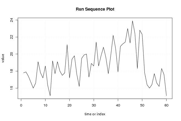
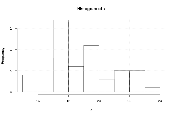
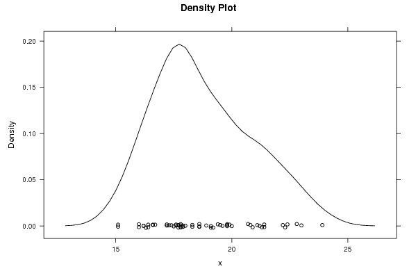
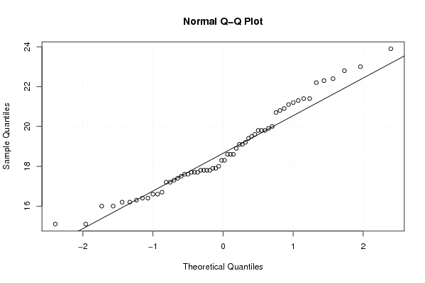
| Dataseries X: | |||||||||||||||||||||||||||||||||||||||||||||||||||||
17,8 17,9 17,4 16,7 16 16,6 19,1 17,8 17,2 18,6 16,3 15,1 19,2 17,7 19,1 18 17,5 17,8 21,1 17,2 19,4 19,8 17,6 16,2 19,5 19,9 20 17,3 18,9 18,6 21,4 18,6 19,8 20,8 19,6 17,7 19,8 22,2 20,7 17,9 20,9 21,2 21,4 23 21,3 23,9 22,4 18,3 22,8 22,3 17,8 16,4 16 16,4 17,7 16,6 16,2 18,3 17,6 15,1 | |||||||||||||||||||||||||||||||||||||||||||||||||||||
Tables (Output of Computation) | |||||||||||||||||||||||||||||||||||||||||||||||||||||
| |||||||||||||||||||||||||||||||||||||||||||||||||||||
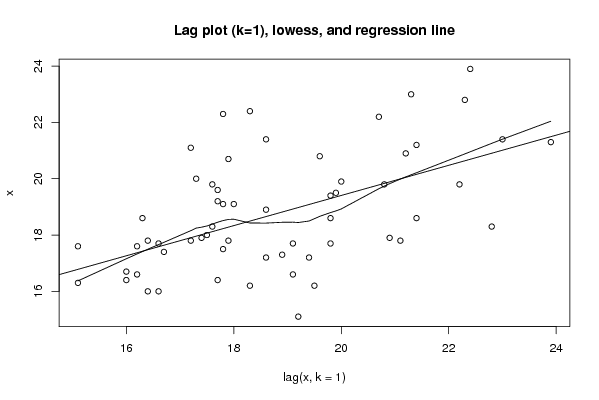
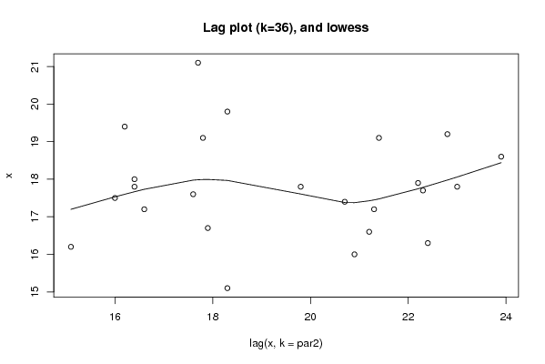
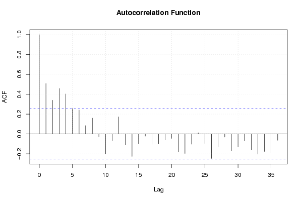
Figures (Output of Computation) | |||||||||||||||||||||||||||||||||||||||||||||||||||||
Input Parameters & R Code | |||||||||||||||||||||||||||||||||||||||||||||||||||||
| Parameters (Session): | |||||||||||||||||||||||||||||||||||||||||||||||||||||
| par1 = 0 ; par2 = 36 ; | |||||||||||||||||||||||||||||||||||||||||||||||||||||
| Parameters (R input): | |||||||||||||||||||||||||||||||||||||||||||||||||||||
| par1 = 0 ; par2 = 36 ; | |||||||||||||||||||||||||||||||||||||||||||||||||||||
| R code (references can be found in the software module): | |||||||||||||||||||||||||||||||||||||||||||||||||||||
par1 <- as.numeric(par1) | |||||||||||||||||||||||||||||||||||||||||||||||||||||