Repository of Reproducible Computations

Free Statistics

of Irreproducible Research!

Author's title

Author

*The author of this computation has been verified*

R Software Module

rwasp_autocorrelation.wasp

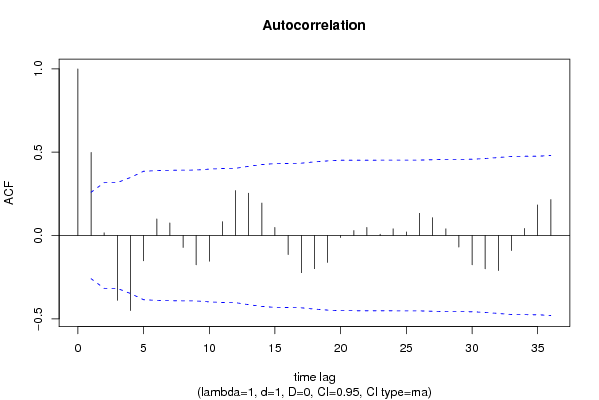
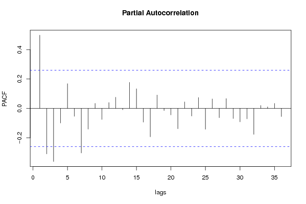
Title produced by software

(Partial) Autocorrelation Function

Date of computation

Fri, 04 Dec 2009 08:00:02 -0700

Cite this page as follows

Statistical Computations at FreeStatistics.org, Office for Research Development and Education, URL https://freestatistics.org/blog/index.php?v=date/2009/Dec/04/t12599388425g7ag9wd8hb63cw.htm/, Retrieved Sat, 27 Apr 2024 13:38:09 +0000

Statistical Computations at FreeStatistics.org, Office for Research Development and Education, URL https://freestatistics.org/blog/index.php?pk=63697, Retrieved Sat, 27 Apr 2024 13:38:09 +0000

QR Codes:

Paste this QR Code to cite your computation.

Original text written by user:

IsPrivate?

No (this computation is public)

User-defined keywords

Estimated Impact

130

Family? (F = Feedback message, R = changed R code, M = changed R Module, P = changed Parameters, D = changed Data)

-     [Univariate Data Series] [data set] [2008-12-01 19:54:57] [b98453cac15ba1066b407e146608df68]
- RMP   [(Partial) Autocorrelation Function] [] [2009-11-27 14:47:30] [b98453cac15ba1066b407e146608df68]
-    D    [(Partial) Autocorrelation Function] [SHW WS9] [2009-12-03 16:22:00] [253127ae8da904b75450fbd69fe4eb21]
-    D        [(Partial) Autocorrelation Function] [ACF] [2009-12-04 15:00:02] [244731fa3e7e6c85774b8c0902c58f85] [Current]
-   PD          [(Partial) Autocorrelation Function] [review WS 9 autoc...] [2009-12-06 20:59:35] [12f02da0296cb21dc23d82ae014a8b71] 
-    D          [(Partial) Autocorrelation Function] [] [2009-12-07 08:45:48] [ade6aa003deff66733e677339d38f25a] 
-   PD            [(Partial) Autocorrelation Function] [rev ws9] [2009-12-07 22:15:45] [6e4e01d7eb22a9f33d58ebb35753a195] 
-   PD            [(Partial) Autocorrelation Function] [] [2009-12-18 02:24:21] [74be16979710d4c4e7c6647856088456] 

Feedback Forum

Post a new message

Dataseries X:

Download CSV

Histogram

Boxplots

6,3
6,2
6,1
6,3
6,5
6,6
6,5
6,2
6,2
5,9
6,1
6,1
6,1
6,1
6,1
6,4
6,7
6,9
7
7
6,8
6,4
5,9
5,5
5,5
5,6
5,8
5,9
6,1
6,1
6
6
5,9
5,5
5,6
5,4
5,2
5,2
5,2
5,5
5,8
5,8
5,5
5,3
5,1
5,2
5,8
5,8
5,5
5
4,9
5,3
6,1
6,5
6,8
6,6
6,4
6,4

Summary of computational transaction
Raw Input	view raw input (R code)
Raw Output	view raw output of R engine
Computing time	2 seconds
R Server	'Gwilym Jenkins' @ 72.249.127.135

\begin{tabular}{lllllllll}
\hline
Summary of computational transaction \tabularnewline
Raw Input & view raw input (R code)  \tabularnewline
Raw Output & view raw output of R engine  \tabularnewline
Computing time & 2 seconds \tabularnewline
R Server & 'Gwilym Jenkins' @ 72.249.127.135 \tabularnewline
\hline
\end{tabular}
%Source: https://freestatistics.org/blog/index.php?pk=63697&T=0

[TABLE]
[ROW][C]Summary of computational transaction[/C][/ROW]
[ROW][C]Raw Input[/C][C]view raw input (R code) [/C][/ROW]
[ROW][C]Raw Output[/C][C]view raw output of R engine [/C][/ROW]
[ROW][C]Computing time[/C][C]2 seconds[/C][/ROW]
[ROW][C]R Server[/C][C]'Gwilym Jenkins' @ 72.249.127.135[/C][/ROW]
[/TABLE]
Source: https://freestatistics.org/blog/index.php?pk=63697&T=0

Globally Unique Identifier (entire table): ba.freestatistics.org/blog/index.php?pk=63697&T=0

As an alternative you can also use a QR Code:

The GUIDs for individual cells are displayed in the table below:

Summary of computational transaction
Raw Input	view raw input (R code)
Raw Output	view raw output of R engine
Computing time	2 seconds
R Server	'Gwilym Jenkins' @ 72.249.127.135

Autocorrelation Function
Time lag k	ACF(k)	T-STAT	P-value
1	0.498596	3.7643	0.000198
2	0.015765	0.119	0.452837
3	-0.389588	-2.9413	0.002358
4	-0.450691	-3.4026	0.000613
5	-0.151777	-1.1459	0.128314
6	0.099228	0.7492	0.228423
7	0.075273	0.5683	0.286033
8	-0.071449	-0.5394	0.295848
9	-0.175828	-1.3275	0.094822
10	-0.154542	-1.1668	0.124082
11	0.082802	0.6251	0.267187
12	0.269757	2.0366	0.023171
13	0.253802	1.9162	0.030182
14	0.195039	1.4725	0.073192
15	0.048411	0.3655	0.358047
16	-0.114264	-0.8627	0.195966
17	-0.22351	-1.6875	0.04849
18	-0.199322	-1.5049	0.068942
19	-0.161848	-1.2219	0.113383
20	-0.012602	-0.0951	0.462268
21	0.029879	0.2256	0.411167
22	0.048218	0.364	0.358588
23	0.007935	0.0599	0.47622
24	0.039982	0.3019	0.381929
25	0.021173	0.1599	0.43678
26	0.133225	1.0058	0.159376
27	0.106603	0.8048	0.21213
28	0.039979	0.3018	0.381939
29	-0.06936	-0.5237	0.301273
30	-0.175986	-1.3287	0.094627
31	-0.199941	-1.5095	0.068344
32	-0.210562	-1.5897	0.058716
33	-0.090698	-0.6848	0.248137
34	0.042688	0.3223	0.374208
35	0.183746	1.3873	0.085383
36	0.215419	1.6264	0.054693

\begin{tabular}{lllllllll}
\hline
Autocorrelation Function \tabularnewline
Time lag k & ACF(k) & T-STAT & P-value \tabularnewline
1 & 0.498596 & 3.7643 & 0.000198 \tabularnewline
2 & 0.015765 & 0.119 & 0.452837 \tabularnewline
3 & -0.389588 & -2.9413 & 0.002358 \tabularnewline
4 & -0.450691 & -3.4026 & 0.000613 \tabularnewline
5 & -0.151777 & -1.1459 & 0.128314 \tabularnewline
6 & 0.099228 & 0.7492 & 0.228423 \tabularnewline
7 & 0.075273 & 0.5683 & 0.286033 \tabularnewline
8 & -0.071449 & -0.5394 & 0.295848 \tabularnewline
9 & -0.175828 & -1.3275 & 0.094822 \tabularnewline
10 & -0.154542 & -1.1668 & 0.124082 \tabularnewline
11 & 0.082802 & 0.6251 & 0.267187 \tabularnewline
12 & 0.269757 & 2.0366 & 0.023171 \tabularnewline
13 & 0.253802 & 1.9162 & 0.030182 \tabularnewline
14 & 0.195039 & 1.4725 & 0.073192 \tabularnewline
15 & 0.048411 & 0.3655 & 0.358047 \tabularnewline
16 & -0.114264 & -0.8627 & 0.195966 \tabularnewline
17 & -0.22351 & -1.6875 & 0.04849 \tabularnewline
18 & -0.199322 & -1.5049 & 0.068942 \tabularnewline
19 & -0.161848 & -1.2219 & 0.113383 \tabularnewline
20 & -0.012602 & -0.0951 & 0.462268 \tabularnewline
21 & 0.029879 & 0.2256 & 0.411167 \tabularnewline
22 & 0.048218 & 0.364 & 0.358588 \tabularnewline
23 & 0.007935 & 0.0599 & 0.47622 \tabularnewline
24 & 0.039982 & 0.3019 & 0.381929 \tabularnewline
25 & 0.021173 & 0.1599 & 0.43678 \tabularnewline
26 & 0.133225 & 1.0058 & 0.159376 \tabularnewline
27 & 0.106603 & 0.8048 & 0.21213 \tabularnewline
28 & 0.039979 & 0.3018 & 0.381939 \tabularnewline
29 & -0.06936 & -0.5237 & 0.301273 \tabularnewline
30 & -0.175986 & -1.3287 & 0.094627 \tabularnewline
31 & -0.199941 & -1.5095 & 0.068344 \tabularnewline
32 & -0.210562 & -1.5897 & 0.058716 \tabularnewline
33 & -0.090698 & -0.6848 & 0.248137 \tabularnewline
34 & 0.042688 & 0.3223 & 0.374208 \tabularnewline
35 & 0.183746 & 1.3873 & 0.085383 \tabularnewline
36 & 0.215419 & 1.6264 & 0.054693 \tabularnewline
\hline
\end{tabular}
%Source: https://freestatistics.org/blog/index.php?pk=63697&T=1

[TABLE]
[ROW][C]Autocorrelation Function[/C][/ROW]
[ROW][C]Time lag k[/C][C]ACF(k)[/C][C]T-STAT[/C][C]P-value[/C][/ROW]
[ROW][C]1[/C][C]0.498596[/C][C]3.7643[/C][C]0.000198[/C][/ROW]
[ROW][C]2[/C][C]0.015765[/C][C]0.119[/C][C]0.452837[/C][/ROW]
[ROW][C]3[/C][C]-0.389588[/C][C]-2.9413[/C][C]0.002358[/C][/ROW]
[ROW][C]4[/C][C]-0.450691[/C][C]-3.4026[/C][C]0.000613[/C][/ROW]
[ROW][C]5[/C][C]-0.151777[/C][C]-1.1459[/C][C]0.128314[/C][/ROW]
[ROW][C]6[/C][C]0.099228[/C][C]0.7492[/C][C]0.228423[/C][/ROW]
[ROW][C]7[/C][C]0.075273[/C][C]0.5683[/C][C]0.286033[/C][/ROW]
[ROW][C]8[/C][C]-0.071449[/C][C]-0.5394[/C][C]0.295848[/C][/ROW]
[ROW][C]9[/C][C]-0.175828[/C][C]-1.3275[/C][C]0.094822[/C][/ROW]
[ROW][C]10[/C][C]-0.154542[/C][C]-1.1668[/C][C]0.124082[/C][/ROW]
[ROW][C]11[/C][C]0.082802[/C][C]0.6251[/C][C]0.267187[/C][/ROW]
[ROW][C]12[/C][C]0.269757[/C][C]2.0366[/C][C]0.023171[/C][/ROW]
[ROW][C]13[/C][C]0.253802[/C][C]1.9162[/C][C]0.030182[/C][/ROW]
[ROW][C]14[/C][C]0.195039[/C][C]1.4725[/C][C]0.073192[/C][/ROW]
[ROW][C]15[/C][C]0.048411[/C][C]0.3655[/C][C]0.358047[/C][/ROW]
[ROW][C]16[/C][C]-0.114264[/C][C]-0.8627[/C][C]0.195966[/C][/ROW]
[ROW][C]17[/C][C]-0.22351[/C][C]-1.6875[/C][C]0.04849[/C][/ROW]
[ROW][C]18[/C][C]-0.199322[/C][C]-1.5049[/C][C]0.068942[/C][/ROW]
[ROW][C]19[/C][C]-0.161848[/C][C]-1.2219[/C][C]0.113383[/C][/ROW]
[ROW][C]20[/C][C]-0.012602[/C][C]-0.0951[/C][C]0.462268[/C][/ROW]
[ROW][C]21[/C][C]0.029879[/C][C]0.2256[/C][C]0.411167[/C][/ROW]
[ROW][C]22[/C][C]0.048218[/C][C]0.364[/C][C]0.358588[/C][/ROW]
[ROW][C]23[/C][C]0.007935[/C][C]0.0599[/C][C]0.47622[/C][/ROW]
[ROW][C]24[/C][C]0.039982[/C][C]0.3019[/C][C]0.381929[/C][/ROW]
[ROW][C]25[/C][C]0.021173[/C][C]0.1599[/C][C]0.43678[/C][/ROW]
[ROW][C]26[/C][C]0.133225[/C][C]1.0058[/C][C]0.159376[/C][/ROW]
[ROW][C]27[/C][C]0.106603[/C][C]0.8048[/C][C]0.21213[/C][/ROW]
[ROW][C]28[/C][C]0.039979[/C][C]0.3018[/C][C]0.381939[/C][/ROW]
[ROW][C]29[/C][C]-0.06936[/C][C]-0.5237[/C][C]0.301273[/C][/ROW]
[ROW][C]30[/C][C]-0.175986[/C][C]-1.3287[/C][C]0.094627[/C][/ROW]
[ROW][C]31[/C][C]-0.199941[/C][C]-1.5095[/C][C]0.068344[/C][/ROW]
[ROW][C]32[/C][C]-0.210562[/C][C]-1.5897[/C][C]0.058716[/C][/ROW]
[ROW][C]33[/C][C]-0.090698[/C][C]-0.6848[/C][C]0.248137[/C][/ROW]
[ROW][C]34[/C][C]0.042688[/C][C]0.3223[/C][C]0.374208[/C][/ROW]
[ROW][C]35[/C][C]0.183746[/C][C]1.3873[/C][C]0.085383[/C][/ROW]
[ROW][C]36[/C][C]0.215419[/C][C]1.6264[/C][C]0.054693[/C][/ROW]
[/TABLE]
Source: https://freestatistics.org/blog/index.php?pk=63697&T=1

Globally Unique Identifier (entire table): ba.freestatistics.org/blog/index.php?pk=63697&T=1

As an alternative you can also use a QR Code:

The GUIDs for individual cells are displayed in the table below:

Autocorrelation Function
Time lag k	ACF(k)	T-STAT	P-value
1	0.498596	3.7643	0.000198
2	0.015765	0.119	0.452837
3	-0.389588	-2.9413	0.002358
4	-0.450691	-3.4026	0.000613
5	-0.151777	-1.1459	0.128314
6	0.099228	0.7492	0.228423
7	0.075273	0.5683	0.286033
8	-0.071449	-0.5394	0.295848
9	-0.175828	-1.3275	0.094822
10	-0.154542	-1.1668	0.124082
11	0.082802	0.6251	0.267187
12	0.269757	2.0366	0.023171
13	0.253802	1.9162	0.030182
14	0.195039	1.4725	0.073192
15	0.048411	0.3655	0.358047
16	-0.114264	-0.8627	0.195966
17	-0.22351	-1.6875	0.04849
18	-0.199322	-1.5049	0.068942
19	-0.161848	-1.2219	0.113383
20	-0.012602	-0.0951	0.462268
21	0.029879	0.2256	0.411167
22	0.048218	0.364	0.358588
23	0.007935	0.0599	0.47622
24	0.039982	0.3019	0.381929
25	0.021173	0.1599	0.43678
26	0.133225	1.0058	0.159376
27	0.106603	0.8048	0.21213
28	0.039979	0.3018	0.381939
29	-0.06936	-0.5237	0.301273
30	-0.175986	-1.3287	0.094627
31	-0.199941	-1.5095	0.068344
32	-0.210562	-1.5897	0.058716
33	-0.090698	-0.6848	0.248137
34	0.042688	0.3223	0.374208
35	0.183746	1.3873	0.085383
36	0.215419	1.6264	0.054693

Partial Autocorrelation Function
Time lag k	PACF(k)	T-STAT	P-value
1	0.498596	3.7643	0.000198
2	-0.309864	-2.3394	0.011421
3	-0.361259	-2.7274	0.004234
4	-0.099182	-0.7488	0.228527
5	0.16862	1.2731	0.104083
6	-0.053586	-0.4046	0.343655
7	-0.303185	-2.289	0.012902
8	-0.140861	-1.0635	0.146025
9	0.034416	0.2598	0.397962
10	-0.074912	-0.5656	0.286952
11	0.039949	0.3016	0.382024
12	0.075993	0.5737	0.284203
13	-0.00914	-0.069	0.472612
14	0.177437	1.3396	0.092843
15	0.133745	1.0098	0.15844
16	-0.093466	-0.7057	0.241638
17	-0.193301	-1.4594	0.074973
18	0.091349	0.6897	0.2466
19	-0.014792	-0.1117	0.455737
20	-0.044166	-0.3334	0.370011
21	-0.138547	-1.046	0.149986
22	0.044159	0.3334	0.37003
23	-0.052185	-0.394	0.347529
24	0.074273	0.5608	0.288583
25	-0.142029	-1.0723	0.144053
26	0.064886	0.4899	0.31305
27	-0.063178	-0.477	0.3176
28	0.067032	0.5061	0.307377
29	-0.068834	-0.5197	0.302646
30	-0.091303	-0.6893	0.246709
31	-0.071117	-0.5369	0.296707
32	-0.176426	-1.332	0.094083
33	0.020194	0.1525	0.439682
34	0.010576	0.0798	0.46832
35	0.03384	0.2555	0.399634
36	-0.055676	-0.4203	0.337908

\begin{tabular}{lllllllll}
\hline
Partial Autocorrelation Function \tabularnewline
Time lag k & PACF(k) & T-STAT & P-value \tabularnewline
1 & 0.498596 & 3.7643 & 0.000198 \tabularnewline
2 & -0.309864 & -2.3394 & 0.011421 \tabularnewline
3 & -0.361259 & -2.7274 & 0.004234 \tabularnewline
4 & -0.099182 & -0.7488 & 0.228527 \tabularnewline
5 & 0.16862 & 1.2731 & 0.104083 \tabularnewline
6 & -0.053586 & -0.4046 & 0.343655 \tabularnewline
7 & -0.303185 & -2.289 & 0.012902 \tabularnewline
8 & -0.140861 & -1.0635 & 0.146025 \tabularnewline
9 & 0.034416 & 0.2598 & 0.397962 \tabularnewline
10 & -0.074912 & -0.5656 & 0.286952 \tabularnewline
11 & 0.039949 & 0.3016 & 0.382024 \tabularnewline
12 & 0.075993 & 0.5737 & 0.284203 \tabularnewline
13 & -0.00914 & -0.069 & 0.472612 \tabularnewline
14 & 0.177437 & 1.3396 & 0.092843 \tabularnewline
15 & 0.133745 & 1.0098 & 0.15844 \tabularnewline
16 & -0.093466 & -0.7057 & 0.241638 \tabularnewline
17 & -0.193301 & -1.4594 & 0.074973 \tabularnewline
18 & 0.091349 & 0.6897 & 0.2466 \tabularnewline
19 & -0.014792 & -0.1117 & 0.455737 \tabularnewline
20 & -0.044166 & -0.3334 & 0.370011 \tabularnewline
21 & -0.138547 & -1.046 & 0.149986 \tabularnewline
22 & 0.044159 & 0.3334 & 0.37003 \tabularnewline
23 & -0.052185 & -0.394 & 0.347529 \tabularnewline
24 & 0.074273 & 0.5608 & 0.288583 \tabularnewline
25 & -0.142029 & -1.0723 & 0.144053 \tabularnewline
26 & 0.064886 & 0.4899 & 0.31305 \tabularnewline
27 & -0.063178 & -0.477 & 0.3176 \tabularnewline
28 & 0.067032 & 0.5061 & 0.307377 \tabularnewline
29 & -0.068834 & -0.5197 & 0.302646 \tabularnewline
30 & -0.091303 & -0.6893 & 0.246709 \tabularnewline
31 & -0.071117 & -0.5369 & 0.296707 \tabularnewline
32 & -0.176426 & -1.332 & 0.094083 \tabularnewline
33 & 0.020194 & 0.1525 & 0.439682 \tabularnewline
34 & 0.010576 & 0.0798 & 0.46832 \tabularnewline
35 & 0.03384 & 0.2555 & 0.399634 \tabularnewline
36 & -0.055676 & -0.4203 & 0.337908 \tabularnewline
\hline
\end{tabular}
%Source: https://freestatistics.org/blog/index.php?pk=63697&T=2

[TABLE]
[ROW][C]Partial Autocorrelation Function[/C][/ROW]
[ROW][C]Time lag k[/C][C]PACF(k)[/C][C]T-STAT[/C][C]P-value[/C][/ROW]
[ROW][C]1[/C][C]0.498596[/C][C]3.7643[/C][C]0.000198[/C][/ROW]
[ROW][C]2[/C][C]-0.309864[/C][C]-2.3394[/C][C]0.011421[/C][/ROW]
[ROW][C]3[/C][C]-0.361259[/C][C]-2.7274[/C][C]0.004234[/C][/ROW]
[ROW][C]4[/C][C]-0.099182[/C][C]-0.7488[/C][C]0.228527[/C][/ROW]
[ROW][C]5[/C][C]0.16862[/C][C]1.2731[/C][C]0.104083[/C][/ROW]
[ROW][C]6[/C][C]-0.053586[/C][C]-0.4046[/C][C]0.343655[/C][/ROW]
[ROW][C]7[/C][C]-0.303185[/C][C]-2.289[/C][C]0.012902[/C][/ROW]
[ROW][C]8[/C][C]-0.140861[/C][C]-1.0635[/C][C]0.146025[/C][/ROW]
[ROW][C]9[/C][C]0.034416[/C][C]0.2598[/C][C]0.397962[/C][/ROW]
[ROW][C]10[/C][C]-0.074912[/C][C]-0.5656[/C][C]0.286952[/C][/ROW]
[ROW][C]11[/C][C]0.039949[/C][C]0.3016[/C][C]0.382024[/C][/ROW]
[ROW][C]12[/C][C]0.075993[/C][C]0.5737[/C][C]0.284203[/C][/ROW]
[ROW][C]13[/C][C]-0.00914[/C][C]-0.069[/C][C]0.472612[/C][/ROW]
[ROW][C]14[/C][C]0.177437[/C][C]1.3396[/C][C]0.092843[/C][/ROW]
[ROW][C]15[/C][C]0.133745[/C][C]1.0098[/C][C]0.15844[/C][/ROW]
[ROW][C]16[/C][C]-0.093466[/C][C]-0.7057[/C][C]0.241638[/C][/ROW]
[ROW][C]17[/C][C]-0.193301[/C][C]-1.4594[/C][C]0.074973[/C][/ROW]
[ROW][C]18[/C][C]0.091349[/C][C]0.6897[/C][C]0.2466[/C][/ROW]
[ROW][C]19[/C][C]-0.014792[/C][C]-0.1117[/C][C]0.455737[/C][/ROW]
[ROW][C]20[/C][C]-0.044166[/C][C]-0.3334[/C][C]0.370011[/C][/ROW]
[ROW][C]21[/C][C]-0.138547[/C][C]-1.046[/C][C]0.149986[/C][/ROW]
[ROW][C]22[/C][C]0.044159[/C][C]0.3334[/C][C]0.37003[/C][/ROW]
[ROW][C]23[/C][C]-0.052185[/C][C]-0.394[/C][C]0.347529[/C][/ROW]
[ROW][C]24[/C][C]0.074273[/C][C]0.5608[/C][C]0.288583[/C][/ROW]
[ROW][C]25[/C][C]-0.142029[/C][C]-1.0723[/C][C]0.144053[/C][/ROW]
[ROW][C]26[/C][C]0.064886[/C][C]0.4899[/C][C]0.31305[/C][/ROW]
[ROW][C]27[/C][C]-0.063178[/C][C]-0.477[/C][C]0.3176[/C][/ROW]
[ROW][C]28[/C][C]0.067032[/C][C]0.5061[/C][C]0.307377[/C][/ROW]
[ROW][C]29[/C][C]-0.068834[/C][C]-0.5197[/C][C]0.302646[/C][/ROW]
[ROW][C]30[/C][C]-0.091303[/C][C]-0.6893[/C][C]0.246709[/C][/ROW]
[ROW][C]31[/C][C]-0.071117[/C][C]-0.5369[/C][C]0.296707[/C][/ROW]
[ROW][C]32[/C][C]-0.176426[/C][C]-1.332[/C][C]0.094083[/C][/ROW]
[ROW][C]33[/C][C]0.020194[/C][C]0.1525[/C][C]0.439682[/C][/ROW]
[ROW][C]34[/C][C]0.010576[/C][C]0.0798[/C][C]0.46832[/C][/ROW]
[ROW][C]35[/C][C]0.03384[/C][C]0.2555[/C][C]0.399634[/C][/ROW]
[ROW][C]36[/C][C]-0.055676[/C][C]-0.4203[/C][C]0.337908[/C][/ROW]
[/TABLE]
Source: https://freestatistics.org/blog/index.php?pk=63697&T=2

Globally Unique Identifier (entire table): ba.freestatistics.org/blog/index.php?pk=63697&T=2

As an alternative you can also use a QR Code:

The GUIDs for individual cells are displayed in the table below:

Partial Autocorrelation Function
Time lag k	PACF(k)	T-STAT	P-value
1	0.498596	3.7643	0.000198
2	-0.309864	-2.3394	0.011421
3	-0.361259	-2.7274	0.004234
4	-0.099182	-0.7488	0.228527
5	0.16862	1.2731	0.104083
6	-0.053586	-0.4046	0.343655
7	-0.303185	-2.289	0.012902
8	-0.140861	-1.0635	0.146025
9	0.034416	0.2598	0.397962
10	-0.074912	-0.5656	0.286952
11	0.039949	0.3016	0.382024
12	0.075993	0.5737	0.284203
13	-0.00914	-0.069	0.472612
14	0.177437	1.3396	0.092843
15	0.133745	1.0098	0.15844
16	-0.093466	-0.7057	0.241638
17	-0.193301	-1.4594	0.074973
18	0.091349	0.6897	0.2466
19	-0.014792	-0.1117	0.455737
20	-0.044166	-0.3334	0.370011
21	-0.138547	-1.046	0.149986
22	0.044159	0.3334	0.37003
23	-0.052185	-0.394	0.347529
24	0.074273	0.5608	0.288583
25	-0.142029	-1.0723	0.144053
26	0.064886	0.4899	0.31305
27	-0.063178	-0.477	0.3176
28	0.067032	0.5061	0.307377
29	-0.068834	-0.5197	0.302646
30	-0.091303	-0.6893	0.246709
31	-0.071117	-0.5369	0.296707
32	-0.176426	-1.332	0.094083
33	0.020194	0.1525	0.439682
34	0.010576	0.0798	0.46832
35	0.03384	0.2555	0.399634
36	-0.055676	-0.4203	0.337908

Figure 1

PNG link

Postscript link

PDF link

Figure 2

PNG link

Postscript link

PDF link

Parameters (Session):

par1 = 36 ; par2 = 1 ; par3 = 1 ; par4 = 0 ; par5 = 12 ; par6 = MA ; par7 = 0.95 ;

Parameters (R input):

par1 = 36 ; par2 = 1 ; par3 = 1 ; par4 = 0 ; par5 = 12 ; par6 = MA ; par7 = 0.95 ;

R code (references can be found in the software module):

if (par1 == 'Default') {
par1 = 10*log10(length(x))
} else {
par1 <- as.numeric(par1)
}
par2 <- as.numeric(par2)
par3 <- as.numeric(par3)
par4 <- as.numeric(par4)
par5 <- as.numeric(par5)
if (par6 == 'White Noise') par6 <- 'white' else par6 <- 'ma'
par7 <- as.numeric(par7)
if (par2 == 0) {
x <- log(x)
} else {
x <- (x ^ par2 - 1) / par2
}
if (par3 > 0) x <- diff(x,lag=1,difference=par3)
if (par4 > 0) x <- diff(x,lag=par5,difference=par4)
bitmap(file='pic1.png')
racf <- acf(x, par1, main='Autocorrelation', xlab='time lag', ylab='ACF', ci.type=par6, ci=par7, sub=paste('(lambda=',par2,', d=',par3,', D=',par4,', CI=', par7, ', CI type=',par6,')',sep=''))
dev.off()
bitmap(file='pic2.png')
rpacf <- pacf(x,par1,main='Partial Autocorrelation',xlab='lags',ylab='PACF')
dev.off()
(myacf <- c(racf$acf))
(mypacf <- c(rpacf$acf))
lengthx <- length(x)
sqrtn <- sqrt(lengthx)
load(file='createtable')
a<-table.start()
a<-table.row.start(a)
a<-table.element(a,'Autocorrelation Function',4,TRUE)
a<-table.row.end(a)
a<-table.row.start(a)
a<-table.element(a,'Time lag k',header=TRUE)
a<-table.element(a,hyperlink('basics.htm','ACF(k)','click here for more information about the Autocorrelation Function'),header=TRUE)
a<-table.element(a,'T-STAT',header=TRUE)
a<-table.element(a,'P-value',header=TRUE)
a<-table.row.end(a)
for (i in 2:(par1+1)) {
a<-table.row.start(a)
a<-table.element(a,i-1,header=TRUE)
a<-table.element(a,round(myacf[i],6))
mytstat <- myacf[i]*sqrtn
a<-table.element(a,round(mytstat,4))
a<-table.element(a,round(1-pt(abs(mytstat),lengthx),6))
a<-table.row.end(a)
}
a<-table.end(a)
table.save(a,file='mytable.tab')
a<-table.start()
a<-table.row.start(a)
a<-table.element(a,'Partial Autocorrelation Function',4,TRUE)
a<-table.row.end(a)
a<-table.row.start(a)
a<-table.element(a,'Time lag k',header=TRUE)
a<-table.element(a,hyperlink('basics.htm','PACF(k)','click here for more information about the Partial Autocorrelation Function'),header=TRUE)
a<-table.element(a,'T-STAT',header=TRUE)
a<-table.element(a,'P-value',header=TRUE)
a<-table.row.end(a)
for (i in 1:par1) {
a<-table.row.start(a)
a<-table.element(a,i,header=TRUE)
a<-table.element(a,round(mypacf[i],6))
mytstat <- mypacf[i]*sqrtn
a<-table.element(a,round(mytstat,4))
a<-table.element(a,round(1-pt(abs(mytstat),lengthx),6))
a<-table.row.end(a)
}
a<-table.end(a)
table.save(a,file='mytable1.tab')

Free Statistics

Description of Statistical Computation

Tree of Dependent Computations

Dataset

Tables (Output of Computation)

Figures (Output of Computation)

Input Parameters & R Code