Free Statistics
of Irreproducible Research!
Description of Statistical Computation | |||||||||||||||||||||
|---|---|---|---|---|---|---|---|---|---|---|---|---|---|---|---|---|---|---|---|---|---|
| Author's title | |||||||||||||||||||||
| Author | *The author of this computation has been verified* | ||||||||||||||||||||
| R Software Module | rwasp_meanplot.wasp | ||||||||||||||||||||
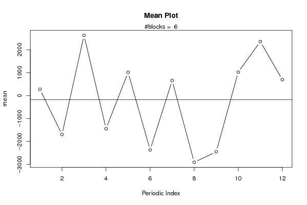
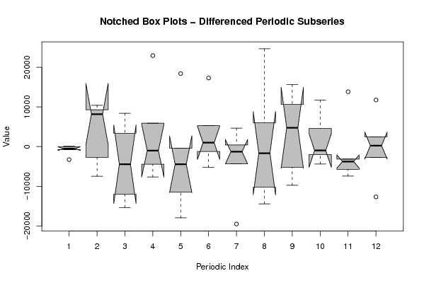
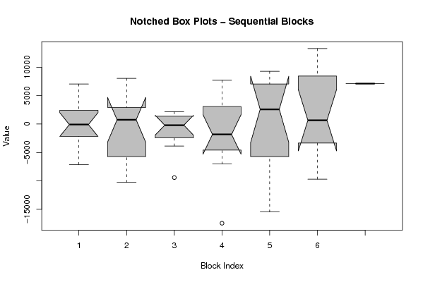
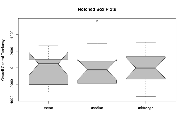
| Title produced by software | Mean Plot | ||||||||||||||||||||
| Date of computation | Fri, 04 Dec 2009 10:33:15 -0700 | ||||||||||||||||||||
| Cite this page as follows | Statistical Computations at FreeStatistics.org, Office for Research Development and Education, URL https://freestatistics.org/blog/index.php?v=date/2009/Dec/04/t12599481268yadroun7rjq4gt.htm/, Retrieved Sun, 28 Apr 2024 06:52:03 +0000 | ||||||||||||||||||||
| Statistical Computations at FreeStatistics.org, Office for Research Development and Education, URL https://freestatistics.org/blog/index.php?pk=63957, Retrieved Sun, 28 Apr 2024 06:52:03 +0000 | |||||||||||||||||||||
| QR Codes: | |||||||||||||||||||||
|
| |||||||||||||||||||||
| Original text written by user: | |||||||||||||||||||||
| IsPrivate? | No (this computation is public) | ||||||||||||||||||||
| User-defined keywords | |||||||||||||||||||||
| Estimated Impact | 146 | ||||||||||||||||||||
Tree of Dependent Computations | |||||||||||||||||||||
| Family? (F = Feedback message, R = changed R code, M = changed R Module, P = changed Parameters, D = changed Data) | |||||||||||||||||||||
| - [Univariate Data Series] [data set] [2008-12-01 19:54:57] [b98453cac15ba1066b407e146608df68] - RMP [ARIMA Backward Selection] [] [2009-11-27 14:53:14] [b98453cac15ba1066b407e146608df68] - D [ARIMA Backward Selection] [BBWS9-Arimabackward1] [2009-12-01 20:26:03] [408e92805dcb18620260f240a7fb9d53] - RM D [Harrell-Davis Quantiles] [BBWS9-Harolddavis] [2009-12-01 20:39:11] [408e92805dcb18620260f240a7fb9d53] - RM [Mean Plot] [BBWS9-Meanplot] [2009-12-01 20:43:16] [408e92805dcb18620260f240a7fb9d53] - PD [Mean Plot] [W9: Mean plot] [2009-12-02 10:46:07] [03d5b865e91ca35b5a5d21b8d6da5aba] - D [Mean Plot] [W9.9] [2009-12-04 17:33:15] [852eae237d08746109043531619a60c9] [Current] | |||||||||||||||||||||
| Feedback Forum | |||||||||||||||||||||
Post a new message | |||||||||||||||||||||
Dataset | |||||||||||||||||||||
| Dataseries X: | |||||||||||||||||||||
-1575.00887827752 -2263.82750005582 7045.75768165492 -2035.83149854133 3886.02985519469 158.539675832947 960.457190377358 -337.841379165606 -7109.61280621946 -7043.92461948593 4685.51755601771 977.408177407792 918.328545859417 589.375354065341 -6891.67878957285 1533.64184150137 2210.55324487903 -9280.29800578057 8034.36112956057 3659.22886246375 7117.41595284467 -2633.18383716224 -4523.01908028135 -10249.2788035485 1517.80356687876 1484.15119995578 -1214.46781890457 2169.24845396691 -2253.92155265332 -2631.74888936717 -3849.26121145593 821.620255775573 -9408.87260464867 1241.88804485160 1179.93724525252 -1962.37832237001 516.653311386494 -2767.97210236296 5629.81911313198 5803.53000967108 -1873.10106680445 -7023.12305076338 -1722.94778568371 -3011.92640473933 -17439.1442995944 -1770.63103827571 -6148.68941133731 7691.62364275427 -4994.18050152824 -4899.69881288656 5524.45031429093 -6451.65580766626 -9155.30558471285 9268.49118895307 4067.36942971564 -15460.4752115729 9214.1160150789 4009.46524142609 8598.3415209042 1171.18094385286 -1585.96191465526 -2329.27119138406 5674.43930504972 -9680.56803374957 13269.3191881056 -4706.51689196404 -3552.85443447458 -3123.75770966460 2912.26032459412 12338.9131048695 10340.0965258702 6543.69991954822 7116.01012281237 | |||||||||||||||||||||
Tables (Output of Computation) | |||||||||||||||||||||
| |||||||||||||||||||||
Figures (Output of Computation) | |||||||||||||||||||||
Input Parameters & R Code | |||||||||||||||||||||
| Parameters (Session): | |||||||||||||||||||||
| par1 = 12 ; | |||||||||||||||||||||
| Parameters (R input): | |||||||||||||||||||||
| par1 = 12 ; | |||||||||||||||||||||
| R code (references can be found in the software module): | |||||||||||||||||||||
par1 <- as.numeric(par1) | |||||||||||||||||||||