Free Statistics
of Irreproducible Research!
Description of Statistical Computation | |||||||||||||||||||||
|---|---|---|---|---|---|---|---|---|---|---|---|---|---|---|---|---|---|---|---|---|---|
| Author's title | |||||||||||||||||||||
| Author | *The author of this computation has been verified* | ||||||||||||||||||||
| R Software Module | rwasp_cloud.wasp | ||||||||||||||||||||
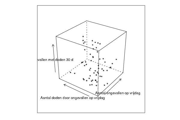
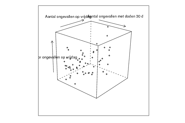
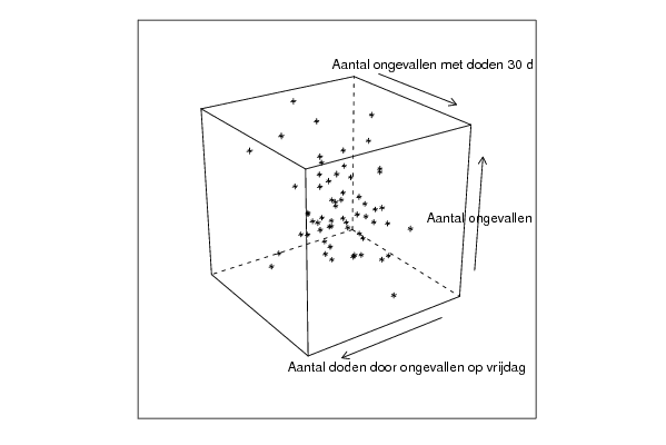
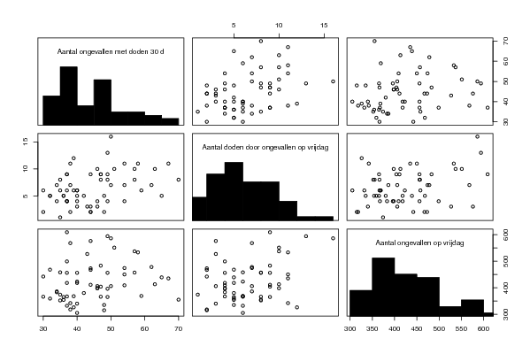
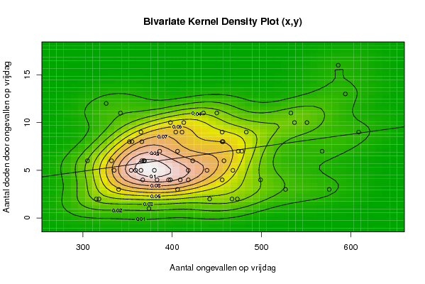
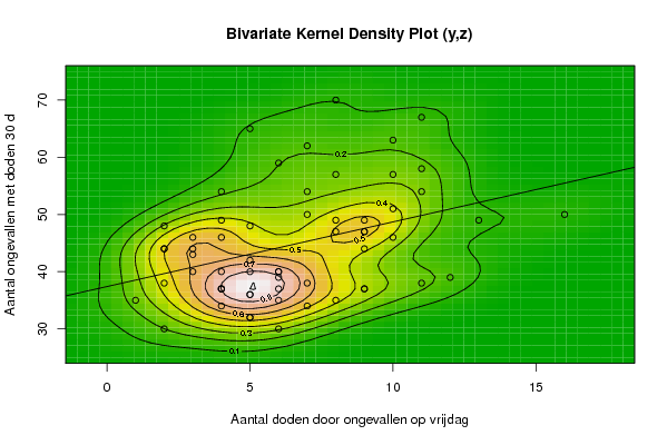
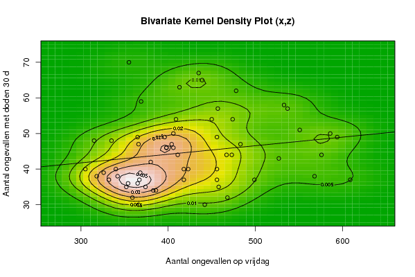
| Title produced by software | Trivariate Scatterplots | ||||||||||||||||||||
| Date of computation | Sat, 05 Dec 2009 06:27:11 -0700 | ||||||||||||||||||||
| Cite this page as follows | Statistical Computations at FreeStatistics.org, Office for Research Development and Education, URL https://freestatistics.org/blog/index.php?v=date/2009/Dec/05/t1260019681u57qv912hjg25vk.htm/, Retrieved Tue, 30 Apr 2024 00:04:20 +0000 | ||||||||||||||||||||
| Statistical Computations at FreeStatistics.org, Office for Research Development and Education, URL https://freestatistics.org/blog/index.php?pk=64245, Retrieved Tue, 30 Apr 2024 00:04:20 +0000 | |||||||||||||||||||||
| QR Codes: | |||||||||||||||||||||
|
| |||||||||||||||||||||
| Original text written by user: | |||||||||||||||||||||
| IsPrivate? | No (this computation is public) | ||||||||||||||||||||
| User-defined keywords | JSSHWPAP5 | ||||||||||||||||||||
| Estimated Impact | 151 | ||||||||||||||||||||
Tree of Dependent Computations | |||||||||||||||||||||
| Family? (F = Feedback message, R = changed R code, M = changed R Module, P = changed Parameters, D = changed Data) | |||||||||||||||||||||
| - [Bivariate Explorative Data Analysis] [Voorspelling model 1] [2009-10-24 11:47:39] [214e6e00abbde49700521a7ef1d30da2] - RMPD [Trivariate Scatterplots] [Trivariate Scatte...] [2009-12-05 13:27:11] [c8fd62404619100d8e91184019148412] [Current] | |||||||||||||||||||||
| Feedback Forum | |||||||||||||||||||||
Post a new message | |||||||||||||||||||||
Dataset | |||||||||||||||||||||
| Dataseries X: | |||||||||||||||||||||
369 380 474 413 537 439 355 473 435 478 450 365 315 340 326 483 406 409 423 404 551 467 332 442 305 368 411 318 398 586 367 383 533 527 418 576 359 342 456 406 374 568 335 458 456 386 457 396 366 499 354 365 594 456 366 398 468 609 418 352 | |||||||||||||||||||||
| Dataseries Y: | |||||||||||||||||||||
6 5 7 10 10 5 8 2 11 7 11 9 2 3 12 9 7 4 6 9 10 2 6 2 6 6 9 2 10 16 4 4 11 3 5 3 5 11 8 3 1 7 5 6 9 7 8 4 6 4 5 5 13 4 8 4 5 9 4 8 | |||||||||||||||||||||
| Dataseries Z: | |||||||||||||||||||||
59 42 54 63 57 65 70 44 67 62 54 49 48 40 39 47 50 54 40 47 51 44 37 30 40 39 44 38 46 50 37 34 58 43 40 44 32 38 49 46 35 38 48 35 37 34 57 49 30 37 36 36 49 40 47 46 32 37 37 35 | |||||||||||||||||||||
Tables (Output of Computation) | |||||||||||||||||||||
| |||||||||||||||||||||
Figures (Output of Computation) | |||||||||||||||||||||
Input Parameters & R Code | |||||||||||||||||||||
| Parameters (Session): | |||||||||||||||||||||
| par1 = 50 ; par2 = 50 ; par3 = Y ; par4 = Y ; par5 = Aantal ongevallen op vrijdag ; par6 = Aantal doden door ongevallen op vrijdag ; par7 = Aantal ongevallen met doden 30 d ; | |||||||||||||||||||||
| Parameters (R input): | |||||||||||||||||||||
| par1 = 50 ; par2 = 50 ; par3 = Y ; par4 = Y ; par5 = Aantal ongevallen op vrijdag ; par6 = Aantal doden door ongevallen op vrijdag ; par7 = Aantal ongevallen met doden 30 d ; | |||||||||||||||||||||
| R code (references can be found in the software module): | |||||||||||||||||||||
x <- array(x,dim=c(length(x),1)) | |||||||||||||||||||||