Free Statistics
of Irreproducible Research!
Description of Statistical Computation | |||||||||||||||||||||
|---|---|---|---|---|---|---|---|---|---|---|---|---|---|---|---|---|---|---|---|---|---|
| Author's title | |||||||||||||||||||||
| Author | *The author of this computation has been verified* | ||||||||||||||||||||
| R Software Module | rwasp_meanplot.wasp | ||||||||||||||||||||
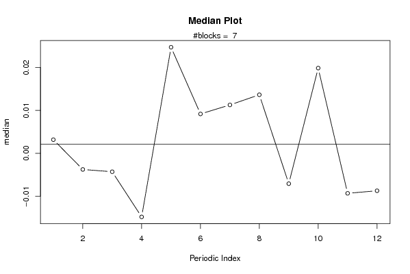
| Title produced by software | Mean Plot | ||||||||||||||||||||
| Date of computation | Mon, 07 Dec 2009 06:06:37 -0700 | ||||||||||||||||||||
| Cite this page as follows | Statistical Computations at FreeStatistics.org, Office for Research Development and Education, URL https://freestatistics.org/blog/index.php?v=date/2009/Dec/07/t12601912392omdsk6fsw3iz9g.htm/, Retrieved Sun, 05 May 2024 03:35:22 +0000 | ||||||||||||||||||||
| Statistical Computations at FreeStatistics.org, Office for Research Development and Education, URL https://freestatistics.org/blog/index.php?pk=64565, Retrieved Sun, 05 May 2024 03:35:22 +0000 | |||||||||||||||||||||
| QR Codes: | |||||||||||||||||||||
|
| |||||||||||||||||||||
| Original text written by user: | |||||||||||||||||||||
| IsPrivate? | No (this computation is public) | ||||||||||||||||||||
| User-defined keywords | |||||||||||||||||||||
| Estimated Impact | 137 | ||||||||||||||||||||
Tree of Dependent Computations | |||||||||||||||||||||
| Family? (F = Feedback message, R = changed R code, M = changed R Module, P = changed Parameters, D = changed Data) | |||||||||||||||||||||
| - [Harrell-Davis Quantiles] [verbetering] [2009-12-07 13:02:33] [408e92805dcb18620260f240a7fb9d53] - RMP [Mean Plot] [verbetering works...] [2009-12-07 13:06:37] [b32ceebc68d054278e6bda97f3d57f91] [Current] | |||||||||||||||||||||
| Feedback Forum | |||||||||||||||||||||
Post a new message | |||||||||||||||||||||
Dataset | |||||||||||||||||||||
| Dataseries X: | |||||||||||||||||||||
0.00450750869087398 -0.0149657506674553 -0.0220859233394083 -0.0148439243168503 0.0676027781490227 0.0264092299234277 -0.0116301716341945 0.0136476387387367 -0.0197271433713688 0.0303927147155863 0.000995418935294206 -0.00874063700973733 -0.0231462237863890 -0.00377238720197872 0.00120873614259887 -0.0176359614054821 0.00250200103515695 -0.0282901697726092 -0.00423879675659204 0.0230884796585779 -0.00859471068972903 0.0198693493392492 -0.0093442264177522 -0.0258281935447543 0.0198614750918193 -0.0122547342511849 -0.00589049815189684 0.0298004421068244 0.0434323456332011 -0.0223164871309812 0.0154280097077713 0.0156548149573578 0.0365282768534479 0.0241846907151588 -0.0322215315404314 -0.0141831668172313 0.0254232968852305 -0.0193736352949016 -0.048536332661388 -0.0766717425093701 0.0281974074828454 0.00917312366714304 0.0616193814776786 -0.0503369625485599 -0.0070958483480044 0.0252260185757131 -0.0147649614724515 0.0297338279951919 0.0427693034085115 0.0334986515495981 -0.00431066374073932 0.0483508046074947 -0.0289633986573534 0.0411760286974008 0.00490436151035459 0.00572516695084428 0.0020827414405662 0.0152702987490803 0.0226514137977885 0.0169257233733748 0.00183213307281401 0.0147224276771016 -0.00123533731905361 0.000655329694370428 -0.00854895738497048 -0.00289709050455367 0.0236354130433993 0.023075931765511 0.0289109594323294 -0.0376782888435601 0.00381606701300569 0.0202008973428546 -0.00412021969633953 0.0418280922509324 0.067769119091173 -0.0525211864056023 0.0247371173448568 0.00923061642650255 0.0112743669564025 -0.000125546542039254 -0.0227570917899331 0.00893231402208485 -0.0388414437336418 -0.0884921733798761 -0.0686977274158266 | |||||||||||||||||||||
Tables (Output of Computation) | |||||||||||||||||||||
| |||||||||||||||||||||
Figures (Output of Computation) | |||||||||||||||||||||
Input Parameters & R Code | |||||||||||||||||||||
| Parameters (Session): | |||||||||||||||||||||
| par1 = 12 ; | |||||||||||||||||||||
| Parameters (R input): | |||||||||||||||||||||
| par1 = 12 ; | |||||||||||||||||||||
| R code (references can be found in the software module): | |||||||||||||||||||||
par1 <- as.numeric(par1) | |||||||||||||||||||||