Free Statistics
of Irreproducible Research!
Description of Statistical Computation | |||||||||||||||||||||
|---|---|---|---|---|---|---|---|---|---|---|---|---|---|---|---|---|---|---|---|---|---|
| Author's title | |||||||||||||||||||||
| Author | *The author of this computation has been verified* | ||||||||||||||||||||
| R Software Module | rwasp_meanplot.wasp | ||||||||||||||||||||
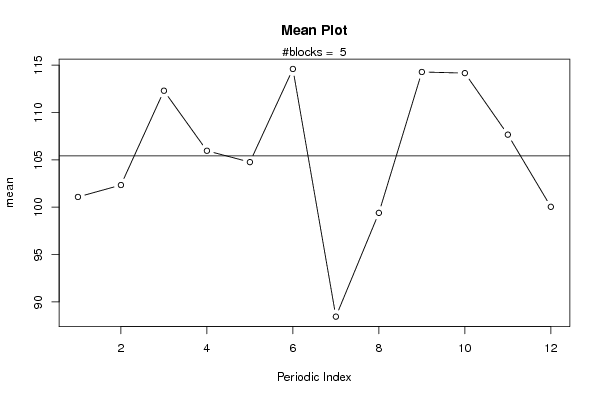
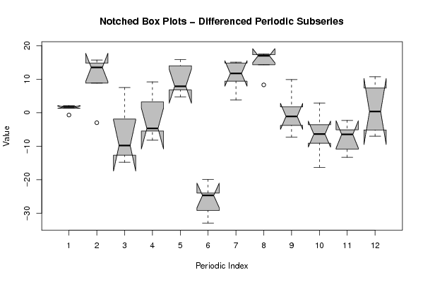
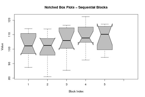
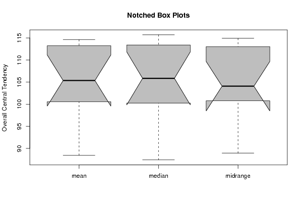
| Title produced by software | Mean Plot | ||||||||||||||||||||
| Date of computation | Wed, 09 Dec 2009 08:08:41 -0700 | ||||||||||||||||||||
| Cite this page as follows | Statistical Computations at FreeStatistics.org, Office for Research Development and Education, URL https://freestatistics.org/blog/index.php?v=date/2009/Dec/09/t126037135905u5509ebrd05qq.htm/, Retrieved Mon, 29 Apr 2024 09:38:11 +0000 | ||||||||||||||||||||
| Statistical Computations at FreeStatistics.org, Office for Research Development and Education, URL https://freestatistics.org/blog/index.php?pk=64985, Retrieved Mon, 29 Apr 2024 09:38:11 +0000 | |||||||||||||||||||||
| QR Codes: | |||||||||||||||||||||
|
| |||||||||||||||||||||
| Original text written by user: | |||||||||||||||||||||
| IsPrivate? | No (this computation is public) | ||||||||||||||||||||
| User-defined keywords | |||||||||||||||||||||
| Estimated Impact | 105 | ||||||||||||||||||||
Tree of Dependent Computations | |||||||||||||||||||||
| Family? (F = Feedback message, R = changed R code, M = changed R Module, P = changed Parameters, D = changed Data) | |||||||||||||||||||||
| - [Mean Plot] [3/11/2009] [2009-11-02 22:07:54] [b98453cac15ba1066b407e146608df68] - PD [Mean Plot] [] [2009-12-09 15:08:41] [9adf7044e3e2072a25a3bb76b79e4d2e] [Current] | |||||||||||||||||||||
| Feedback Forum | |||||||||||||||||||||
Post a new message | |||||||||||||||||||||
Dataset | |||||||||||||||||||||
| Dataseries X: | |||||||||||||||||||||
95.1 97.0 112.7 102.9 97.4 111.4 87.4 96.8 114.1 110.3 103.9 101.6 94.6 95.9 104.7 102.8 98.1 113.9 80.9 95.7 113.2 105.9 108.8 102.3 99.0 100.7 115.5 100.7 109.9 114.6 85.4 100.5 114.8 116.5 112.9 102.0 106.0 105.3 118.8 106.1 109.3 117.2 92.5 104.2 112.5 122.4 113.3 100.0 110.7 112.8 109.8 117.3 109.1 115.9 96.0 99.8 116.8 115.7 99.4 94.3 | |||||||||||||||||||||
Tables (Output of Computation) | |||||||||||||||||||||
| |||||||||||||||||||||
Figures (Output of Computation) | |||||||||||||||||||||
Input Parameters & R Code | |||||||||||||||||||||
| Parameters (Session): | |||||||||||||||||||||
| par1 = 12 ; | |||||||||||||||||||||
| Parameters (R input): | |||||||||||||||||||||
| par1 = 12 ; | |||||||||||||||||||||
| R code (references can be found in the software module): | |||||||||||||||||||||
par1 <- as.numeric(par1) | |||||||||||||||||||||