Free Statistics
of Irreproducible Research!
Description of Statistical Computation | |||||||||||||||||||||||||||||||||||||||||||||||||||||
|---|---|---|---|---|---|---|---|---|---|---|---|---|---|---|---|---|---|---|---|---|---|---|---|---|---|---|---|---|---|---|---|---|---|---|---|---|---|---|---|---|---|---|---|---|---|---|---|---|---|---|---|---|---|
| Author's title | |||||||||||||||||||||||||||||||||||||||||||||||||||||
| Author | *The author of this computation has been verified* | ||||||||||||||||||||||||||||||||||||||||||||||||||||
| R Software Module | rwasp_edauni.wasp | ||||||||||||||||||||||||||||||||||||||||||||||||||||
| Title produced by software | Univariate Explorative Data Analysis | ||||||||||||||||||||||||||||||||||||||||||||||||||||
| Date of computation | Wed, 09 Dec 2009 11:05:38 -0700 | ||||||||||||||||||||||||||||||||||||||||||||||||||||
| Cite this page as follows | Statistical Computations at FreeStatistics.org, Office for Research Development and Education, URL https://freestatistics.org/blog/index.php?v=date/2009/Dec/09/t12603820485dugmt1eb3f786b.htm/, Retrieved Mon, 29 Apr 2024 10:02:59 +0000 | ||||||||||||||||||||||||||||||||||||||||||||||||||||
| Statistical Computations at FreeStatistics.org, Office for Research Development and Education, URL https://freestatistics.org/blog/index.php?pk=65107, Retrieved Mon, 29 Apr 2024 10:02:59 +0000 | |||||||||||||||||||||||||||||||||||||||||||||||||||||
| QR Codes: | |||||||||||||||||||||||||||||||||||||||||||||||||||||
|
| |||||||||||||||||||||||||||||||||||||||||||||||||||||
| Original text written by user: | |||||||||||||||||||||||||||||||||||||||||||||||||||||
| IsPrivate? | No (this computation is public) | ||||||||||||||||||||||||||||||||||||||||||||||||||||
| User-defined keywords | |||||||||||||||||||||||||||||||||||||||||||||||||||||
| Estimated Impact | 102 | ||||||||||||||||||||||||||||||||||||||||||||||||||||
Tree of Dependent Computations | |||||||||||||||||||||||||||||||||||||||||||||||||||||
| Family? (F = Feedback message, R = changed R code, M = changed R Module, P = changed Parameters, D = changed Data) | |||||||||||||||||||||||||||||||||||||||||||||||||||||
| - [Univariate Explorative Data Analysis] [cs.shw.paper.univ...] [2009-12-09 18:05:38] [d41d8cd98f00b204e9800998ecf8427e] [Current] | |||||||||||||||||||||||||||||||||||||||||||||||||||||
| Feedback Forum | |||||||||||||||||||||||||||||||||||||||||||||||||||||
Post a new message | |||||||||||||||||||||||||||||||||||||||||||||||||||||
Dataset | |||||||||||||||||||||||||||||||||||||||||||||||||||||
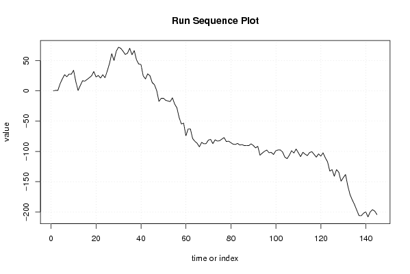
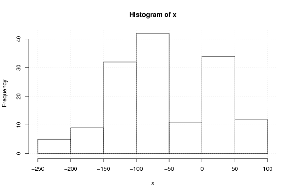
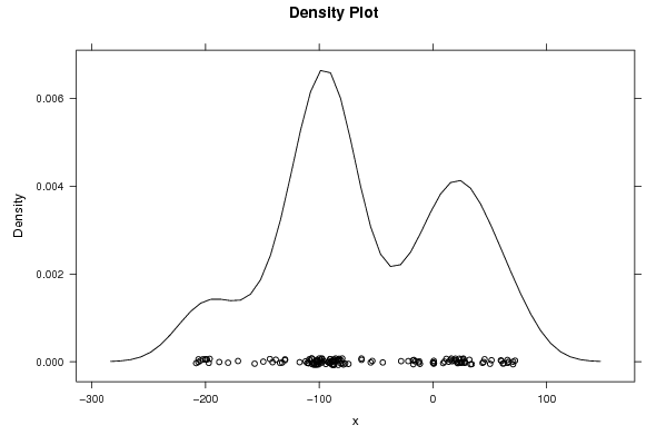
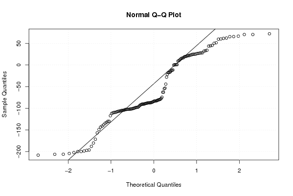
| Dataseries X: | |||||||||||||||||||||||||||||||||||||||||||||||||||||
0,00 0,91 0,74 11,74 19,90 26,77 23,42 27,86 27,69 34,12 15,35 0,65 8,98 16,83 16,16 18,91 21,80 24,98 32,07 23,12 25,50 21,19 26,70 21,78 33,04 45,41 61,55 50,24 65,51 72,17 70,44 65,69 60,25 62,31 70,48 59,73 66,68 51,51 44,46 43,64 24,83 19,80 28,22 24,97 13,84 10,17 0,60 -17,28 -12,31 -12,14 -15,49 -16,70 -17,62 -11,45 -21,71 -28,00 -44,11 -54,76 -53,32 -74,29 -62,78 -62,86 -78,74 -83,31 -86,54 -92,44 -85,10 -87,44 -87,17 -81,37 -80,09 -87,23 -80,88 -82,93 -82,43 -79,69 -77,21 -83,69 -83,13 -85,59 -88,00 -88,56 -86,82 -89,51 -88,74 -90,44 -90,19 -90,47 -87,50 -90,17 -94,16 -91,67 -106,39 -102,77 -99,88 -97,77 -102,14 -101,64 -105,13 -99,01 -97,59 -97,65 -101,12 -109,59 -111,95 -106,19 -98,80 -102,68 -96,07 -102,28 -108,71 -101,48 -104,53 -106,94 -101,89 -100,37 -104,90 -109,43 -104,06 -107,85 -102,33 -110,65 -117,22 -132,60 -130,09 -141,03 -130,06 -134,47 -149,17 -143,39 -138,20 -156,80 -171,42 -180,18 -187,92 -197,15 -206,14 -206,31 -202,25 -199,91 -208,24 -199,96 -196,32 -198,68 -204,45 | |||||||||||||||||||||||||||||||||||||||||||||||||||||
Tables (Output of Computation) | |||||||||||||||||||||||||||||||||||||||||||||||||||||
| |||||||||||||||||||||||||||||||||||||||||||||||||||||
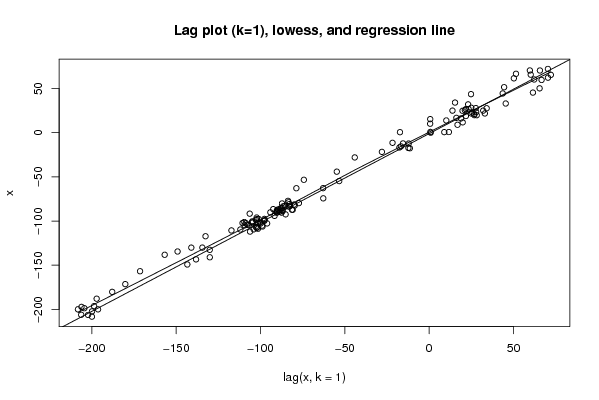
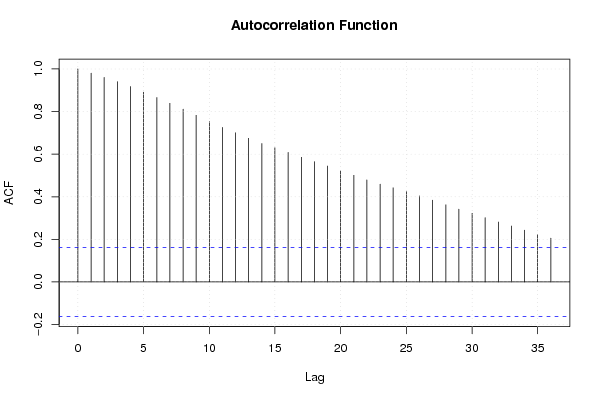
Figures (Output of Computation) | |||||||||||||||||||||||||||||||||||||||||||||||||||||
Input Parameters & R Code | |||||||||||||||||||||||||||||||||||||||||||||||||||||
| Parameters (Session): | |||||||||||||||||||||||||||||||||||||||||||||||||||||
| par1 = 0 ; par2 = 36 ; | |||||||||||||||||||||||||||||||||||||||||||||||||||||
| Parameters (R input): | |||||||||||||||||||||||||||||||||||||||||||||||||||||
| par1 = 0 ; par2 = 36 ; | |||||||||||||||||||||||||||||||||||||||||||||||||||||
| R code (references can be found in the software module): | |||||||||||||||||||||||||||||||||||||||||||||||||||||
par1 <- as.numeric(par1) | |||||||||||||||||||||||||||||||||||||||||||||||||||||