Repository of Reproducible Computations

Free Statistics

of Irreproducible Research!

Author's title

Author

*Unverified author*

R Software Module

rwasp_autocorrelation.wasp

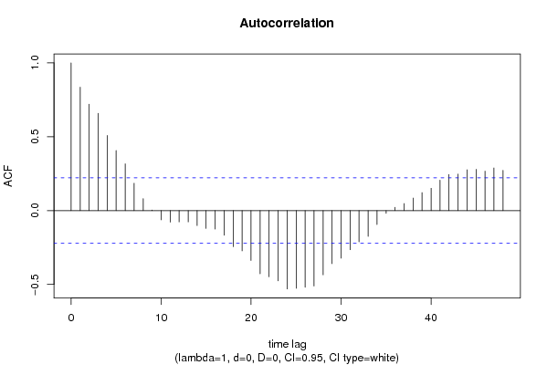
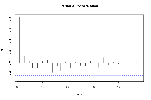
Title produced by software

(Partial) Autocorrelation Function

Date of computation

Sun, 13 Dec 2009 07:36:32 -0700

Cite this page as follows

Statistical Computations at FreeStatistics.org, Office for Research Development and Education, URL https://freestatistics.org/blog/index.php?v=date/2009/Dec/13/t1260715040pi7fio0yb7ekhoz.htm/, Retrieved Sun, 28 Apr 2024 08:10:34 +0000

Statistical Computations at FreeStatistics.org, Office for Research Development and Education, URL https://freestatistics.org/blog/index.php?pk=67303, Retrieved Sun, 28 Apr 2024 08:10:34 +0000

QR Codes:

Paste this QR Code to cite your computation.

Original text written by user:

IsPrivate?

No (this computation is public)

User-defined keywords

KDGP2W21

Estimated Impact

118

Family? (F = Feedback message, R = changed R code, M = changed R Module, P = changed Parameters, D = changed Data)

-     [Bootstrap Plot - Central Tendency] [Bootstrap Plot ma...] [2009-12-13 13:46:28] [2111252d51b8b4a3589bda750b6f824c]
- RMPD    [(Partial) Autocorrelation Function] [autocorrelation cola] [2009-12-13 14:36:32] [257e61bb186fb77667d40c094d5abaa7] [Current]

Feedback Forum

Post a new message

Dataseries X:

Download CSV

Histogram

Boxplots

1,25
1,25
1,26
1,26
1,26
1,26
1,27
1,27
1,29
1,31
1,32
1,32
1,33
1,33
1,32
1,32
1,31
1,3
1,31
1,29
1,3
1,3
1,32
1,31
1,35
1,35
1,36
1,37
1,37
1,37
1,32
1,32
1,31
1,31
1,34
1,31
1,26
1,27
1,24
1,25
1,27
1,25
1,26
1,27
1,26
1,26
1,28
1,27
1,28
1,27
1,26
1,27
1,27
1,28
1,27
1,26
1,3
1,31
1,28
1,29
1,31
1,29
1,29
1,32
1,3
1,29
1,31
1,29
1,33
1,35
1,32
1,33
1,34
1,34
1,33
1,33
1,35
1,32

Summary of computational transaction
Raw Input	view raw input (R code)
Raw Output	view raw output of R engine
Computing time	1 seconds
R Server	'Gwilym Jenkins' @ 72.249.127.135

\begin{tabular}{lllllllll}
\hline
Summary of computational transaction \tabularnewline
Raw Input & view raw input (R code)  \tabularnewline
Raw Output & view raw output of R engine  \tabularnewline
Computing time & 1 seconds \tabularnewline
R Server & 'Gwilym Jenkins' @ 72.249.127.135 \tabularnewline
\hline
\end{tabular}
%Source: https://freestatistics.org/blog/index.php?pk=67303&T=0

[TABLE]
[ROW][C]Summary of computational transaction[/C][/ROW]
[ROW][C]Raw Input[/C][C]view raw input (R code) [/C][/ROW]
[ROW][C]Raw Output[/C][C]view raw output of R engine [/C][/ROW]
[ROW][C]Computing time[/C][C]1 seconds[/C][/ROW]
[ROW][C]R Server[/C][C]'Gwilym Jenkins' @ 72.249.127.135[/C][/ROW]
[/TABLE]
Source: https://freestatistics.org/blog/index.php?pk=67303&T=0

Globally Unique Identifier (entire table): ba.freestatistics.org/blog/index.php?pk=67303&T=0

As an alternative you can also use a QR Code:

The GUIDs for individual cells are displayed in the table below:

Summary of computational transaction
Raw Input	view raw input (R code)
Raw Output	view raw output of R engine
Computing time	1 seconds
R Server	'Gwilym Jenkins' @ 72.249.127.135

Autocorrelation Function
Time lag k	ACF(k)	T-STAT	P-value
1	0.835447	7.3785	0
2	0.720487	6.3632	0
3	0.658919	5.8194	0
4	0.508466	4.4906	1.2e-05
5	0.406542	3.5905	0.000287
6	0.31647	2.795	0.003265
7	0.184918	1.6332	0.053234
8	0.080685	0.7126	0.239113
9	0.003406	0.0301	0.48804
10	-0.063207	-0.5582	0.289143
11	-0.078678	-0.6949	0.244603
12	-0.076493	-0.6756	0.250657
13	-0.076618	-0.6767	0.250309
14	-0.101691	-0.8981	0.185946
15	-0.120899	-1.0677	0.144464
16	-0.125703	-1.1102	0.135166
17	-0.167186	-1.4765	0.071912
18	-0.244282	-2.1574	0.017025
19	-0.272728	-2.4087	0.009185
20	-0.337731	-2.9828	0.001906
21	-0.427864	-3.7788	0.000153
22	-0.448014	-3.9568	8.3e-05
23	-0.476339	-4.2069	3.4e-05
24	-0.530736	-4.6873	6e-06
25	-0.526181	-4.6471	7e-06
26	-0.519195	-4.5854	8e-06
27	-0.511085	-4.5138	1.1e-05
28	-0.435422	-3.8455	0.000122
29	-0.359821	-3.1778	0.001064
30	-0.322204	-2.8456	0.00283
31	-0.26526	-2.3427	0.010847
32	-0.211933	-1.8717	0.032496
33	-0.175015	-1.5457	0.063114
34	-0.094247	-0.8324	0.203871
35	-0.018463	-0.1631	0.435445
36	0.02201	0.1944	0.423189
37	0.047442	0.419	0.338187
38	0.084542	0.7467	0.228759
39	0.121946	1.077	0.1424
40	0.151054	1.3341	0.09303
41	0.205932	1.8187	0.036395
42	0.244399	2.1585	0.016983
43	0.246949	2.181	0.016099
44	0.276513	2.4421	0.008433
45	0.279062	2.4646	0.007957
46	0.26739	2.3615	0.010348
47	0.288719	2.5499	0.006368
48	0.272185	2.4039	0.009298

\begin{tabular}{lllllllll}
\hline
Autocorrelation Function \tabularnewline
Time lag k & ACF(k) & T-STAT & P-value \tabularnewline
1 & 0.835447 & 7.3785 & 0 \tabularnewline
2 & 0.720487 & 6.3632 & 0 \tabularnewline
3 & 0.658919 & 5.8194 & 0 \tabularnewline
4 & 0.508466 & 4.4906 & 1.2e-05 \tabularnewline
5 & 0.406542 & 3.5905 & 0.000287 \tabularnewline
6 & 0.31647 & 2.795 & 0.003265 \tabularnewline
7 & 0.184918 & 1.6332 & 0.053234 \tabularnewline
8 & 0.080685 & 0.7126 & 0.239113 \tabularnewline
9 & 0.003406 & 0.0301 & 0.48804 \tabularnewline
10 & -0.063207 & -0.5582 & 0.289143 \tabularnewline
11 & -0.078678 & -0.6949 & 0.244603 \tabularnewline
12 & -0.076493 & -0.6756 & 0.250657 \tabularnewline
13 & -0.076618 & -0.6767 & 0.250309 \tabularnewline
14 & -0.101691 & -0.8981 & 0.185946 \tabularnewline
15 & -0.120899 & -1.0677 & 0.144464 \tabularnewline
16 & -0.125703 & -1.1102 & 0.135166 \tabularnewline
17 & -0.167186 & -1.4765 & 0.071912 \tabularnewline
18 & -0.244282 & -2.1574 & 0.017025 \tabularnewline
19 & -0.272728 & -2.4087 & 0.009185 \tabularnewline
20 & -0.337731 & -2.9828 & 0.001906 \tabularnewline
21 & -0.427864 & -3.7788 & 0.000153 \tabularnewline
22 & -0.448014 & -3.9568 & 8.3e-05 \tabularnewline
23 & -0.476339 & -4.2069 & 3.4e-05 \tabularnewline
24 & -0.530736 & -4.6873 & 6e-06 \tabularnewline
25 & -0.526181 & -4.6471 & 7e-06 \tabularnewline
26 & -0.519195 & -4.5854 & 8e-06 \tabularnewline
27 & -0.511085 & -4.5138 & 1.1e-05 \tabularnewline
28 & -0.435422 & -3.8455 & 0.000122 \tabularnewline
29 & -0.359821 & -3.1778 & 0.001064 \tabularnewline
30 & -0.322204 & -2.8456 & 0.00283 \tabularnewline
31 & -0.26526 & -2.3427 & 0.010847 \tabularnewline
32 & -0.211933 & -1.8717 & 0.032496 \tabularnewline
33 & -0.175015 & -1.5457 & 0.063114 \tabularnewline
34 & -0.094247 & -0.8324 & 0.203871 \tabularnewline
35 & -0.018463 & -0.1631 & 0.435445 \tabularnewline
36 & 0.02201 & 0.1944 & 0.423189 \tabularnewline
37 & 0.047442 & 0.419 & 0.338187 \tabularnewline
38 & 0.084542 & 0.7467 & 0.228759 \tabularnewline
39 & 0.121946 & 1.077 & 0.1424 \tabularnewline
40 & 0.151054 & 1.3341 & 0.09303 \tabularnewline
41 & 0.205932 & 1.8187 & 0.036395 \tabularnewline
42 & 0.244399 & 2.1585 & 0.016983 \tabularnewline
43 & 0.246949 & 2.181 & 0.016099 \tabularnewline
44 & 0.276513 & 2.4421 & 0.008433 \tabularnewline
45 & 0.279062 & 2.4646 & 0.007957 \tabularnewline
46 & 0.26739 & 2.3615 & 0.010348 \tabularnewline
47 & 0.288719 & 2.5499 & 0.006368 \tabularnewline
48 & 0.272185 & 2.4039 & 0.009298 \tabularnewline
\hline
\end{tabular}
%Source: https://freestatistics.org/blog/index.php?pk=67303&T=1

[TABLE]
[ROW][C]Autocorrelation Function[/C][/ROW]
[ROW][C]Time lag k[/C][C]ACF(k)[/C][C]T-STAT[/C][C]P-value[/C][/ROW]
[ROW][C]1[/C][C]0.835447[/C][C]7.3785[/C][C]0[/C][/ROW]
[ROW][C]2[/C][C]0.720487[/C][C]6.3632[/C][C]0[/C][/ROW]
[ROW][C]3[/C][C]0.658919[/C][C]5.8194[/C][C]0[/C][/ROW]
[ROW][C]4[/C][C]0.508466[/C][C]4.4906[/C][C]1.2e-05[/C][/ROW]
[ROW][C]5[/C][C]0.406542[/C][C]3.5905[/C][C]0.000287[/C][/ROW]
[ROW][C]6[/C][C]0.31647[/C][C]2.795[/C][C]0.003265[/C][/ROW]
[ROW][C]7[/C][C]0.184918[/C][C]1.6332[/C][C]0.053234[/C][/ROW]
[ROW][C]8[/C][C]0.080685[/C][C]0.7126[/C][C]0.239113[/C][/ROW]
[ROW][C]9[/C][C]0.003406[/C][C]0.0301[/C][C]0.48804[/C][/ROW]
[ROW][C]10[/C][C]-0.063207[/C][C]-0.5582[/C][C]0.289143[/C][/ROW]
[ROW][C]11[/C][C]-0.078678[/C][C]-0.6949[/C][C]0.244603[/C][/ROW]
[ROW][C]12[/C][C]-0.076493[/C][C]-0.6756[/C][C]0.250657[/C][/ROW]
[ROW][C]13[/C][C]-0.076618[/C][C]-0.6767[/C][C]0.250309[/C][/ROW]
[ROW][C]14[/C][C]-0.101691[/C][C]-0.8981[/C][C]0.185946[/C][/ROW]
[ROW][C]15[/C][C]-0.120899[/C][C]-1.0677[/C][C]0.144464[/C][/ROW]
[ROW][C]16[/C][C]-0.125703[/C][C]-1.1102[/C][C]0.135166[/C][/ROW]
[ROW][C]17[/C][C]-0.167186[/C][C]-1.4765[/C][C]0.071912[/C][/ROW]
[ROW][C]18[/C][C]-0.244282[/C][C]-2.1574[/C][C]0.017025[/C][/ROW]
[ROW][C]19[/C][C]-0.272728[/C][C]-2.4087[/C][C]0.009185[/C][/ROW]
[ROW][C]20[/C][C]-0.337731[/C][C]-2.9828[/C][C]0.001906[/C][/ROW]
[ROW][C]21[/C][C]-0.427864[/C][C]-3.7788[/C][C]0.000153[/C][/ROW]
[ROW][C]22[/C][C]-0.448014[/C][C]-3.9568[/C][C]8.3e-05[/C][/ROW]
[ROW][C]23[/C][C]-0.476339[/C][C]-4.2069[/C][C]3.4e-05[/C][/ROW]
[ROW][C]24[/C][C]-0.530736[/C][C]-4.6873[/C][C]6e-06[/C][/ROW]
[ROW][C]25[/C][C]-0.526181[/C][C]-4.6471[/C][C]7e-06[/C][/ROW]
[ROW][C]26[/C][C]-0.519195[/C][C]-4.5854[/C][C]8e-06[/C][/ROW]
[ROW][C]27[/C][C]-0.511085[/C][C]-4.5138[/C][C]1.1e-05[/C][/ROW]
[ROW][C]28[/C][C]-0.435422[/C][C]-3.8455[/C][C]0.000122[/C][/ROW]
[ROW][C]29[/C][C]-0.359821[/C][C]-3.1778[/C][C]0.001064[/C][/ROW]
[ROW][C]30[/C][C]-0.322204[/C][C]-2.8456[/C][C]0.00283[/C][/ROW]
[ROW][C]31[/C][C]-0.26526[/C][C]-2.3427[/C][C]0.010847[/C][/ROW]
[ROW][C]32[/C][C]-0.211933[/C][C]-1.8717[/C][C]0.032496[/C][/ROW]
[ROW][C]33[/C][C]-0.175015[/C][C]-1.5457[/C][C]0.063114[/C][/ROW]
[ROW][C]34[/C][C]-0.094247[/C][C]-0.8324[/C][C]0.203871[/C][/ROW]
[ROW][C]35[/C][C]-0.018463[/C][C]-0.1631[/C][C]0.435445[/C][/ROW]
[ROW][C]36[/C][C]0.02201[/C][C]0.1944[/C][C]0.423189[/C][/ROW]
[ROW][C]37[/C][C]0.047442[/C][C]0.419[/C][C]0.338187[/C][/ROW]
[ROW][C]38[/C][C]0.084542[/C][C]0.7467[/C][C]0.228759[/C][/ROW]
[ROW][C]39[/C][C]0.121946[/C][C]1.077[/C][C]0.1424[/C][/ROW]
[ROW][C]40[/C][C]0.151054[/C][C]1.3341[/C][C]0.09303[/C][/ROW]
[ROW][C]41[/C][C]0.205932[/C][C]1.8187[/C][C]0.036395[/C][/ROW]
[ROW][C]42[/C][C]0.244399[/C][C]2.1585[/C][C]0.016983[/C][/ROW]
[ROW][C]43[/C][C]0.246949[/C][C]2.181[/C][C]0.016099[/C][/ROW]
[ROW][C]44[/C][C]0.276513[/C][C]2.4421[/C][C]0.008433[/C][/ROW]
[ROW][C]45[/C][C]0.279062[/C][C]2.4646[/C][C]0.007957[/C][/ROW]
[ROW][C]46[/C][C]0.26739[/C][C]2.3615[/C][C]0.010348[/C][/ROW]
[ROW][C]47[/C][C]0.288719[/C][C]2.5499[/C][C]0.006368[/C][/ROW]
[ROW][C]48[/C][C]0.272185[/C][C]2.4039[/C][C]0.009298[/C][/ROW]
[/TABLE]
Source: https://freestatistics.org/blog/index.php?pk=67303&T=1

Globally Unique Identifier (entire table): ba.freestatistics.org/blog/index.php?pk=67303&T=1

As an alternative you can also use a QR Code:

The GUIDs for individual cells are displayed in the table below:

Autocorrelation Function
Time lag k	ACF(k)	T-STAT	P-value
1	0.835447	7.3785	0
2	0.720487	6.3632	0
3	0.658919	5.8194	0
4	0.508466	4.4906	1.2e-05
5	0.406542	3.5905	0.000287
6	0.31647	2.795	0.003265
7	0.184918	1.6332	0.053234
8	0.080685	0.7126	0.239113
9	0.003406	0.0301	0.48804
10	-0.063207	-0.5582	0.289143
11	-0.078678	-0.6949	0.244603
12	-0.076493	-0.6756	0.250657
13	-0.076618	-0.6767	0.250309
14	-0.101691	-0.8981	0.185946
15	-0.120899	-1.0677	0.144464
16	-0.125703	-1.1102	0.135166
17	-0.167186	-1.4765	0.071912
18	-0.244282	-2.1574	0.017025
19	-0.272728	-2.4087	0.009185
20	-0.337731	-2.9828	0.001906
21	-0.427864	-3.7788	0.000153
22	-0.448014	-3.9568	8.3e-05
23	-0.476339	-4.2069	3.4e-05
24	-0.530736	-4.6873	6e-06
25	-0.526181	-4.6471	7e-06
26	-0.519195	-4.5854	8e-06
27	-0.511085	-4.5138	1.1e-05
28	-0.435422	-3.8455	0.000122
29	-0.359821	-3.1778	0.001064
30	-0.322204	-2.8456	0.00283
31	-0.26526	-2.3427	0.010847
32	-0.211933	-1.8717	0.032496
33	-0.175015	-1.5457	0.063114
34	-0.094247	-0.8324	0.203871
35	-0.018463	-0.1631	0.435445
36	0.02201	0.1944	0.423189
37	0.047442	0.419	0.338187
38	0.084542	0.7467	0.228759
39	0.121946	1.077	0.1424
40	0.151054	1.3341	0.09303
41	0.205932	1.8187	0.036395
42	0.244399	2.1585	0.016983
43	0.246949	2.181	0.016099
44	0.276513	2.4421	0.008433
45	0.279062	2.4646	0.007957
46	0.26739	2.3615	0.010348
47	0.288719	2.5499	0.006368
48	0.272185	2.4039	0.009298

Partial Autocorrelation Function
Time lag k	PACF(k)	T-STAT	P-value
1	0.835447	7.3785	0
2	0.074547	0.6584	0.256117
3	0.131785	1.1639	0.124008
4	-0.28771	-2.541	0.006519
5	0.035147	0.3104	0.37854
6	-0.086356	-0.7627	0.22398
7	-0.111799	-0.9874	0.163253
8	-0.083926	-0.7412	0.230395
9	-0.004571	-0.0404	0.483949
10	0.030982	0.2736	0.392546
11	0.118159	1.0435	0.149959
12	0.055512	0.4903	0.312659
13	0.024427	0.2157	0.41488
14	-0.167441	-1.4788	0.07161
15	-0.066427	-0.5867	0.279562
16	-0.044813	-0.3958	0.346674
17	-0.140104	-1.2374	0.109831
18	-0.25255	-2.2305	0.014295
19	0.027052	0.2389	0.405899
20	-0.119555	-1.0559	0.147142
21	-0.091426	-0.8075	0.21093
22	0.023672	0.2091	0.417472
23	0.0114	0.1007	0.460029
24	-0.148467	-1.3112	0.096814
25	-0.041156	-0.3635	0.358615
26	-0.073865	-0.6524	0.258045
27	-0.042823	-0.3782	0.353154
28	0.011893	0.105	0.45831
29	0.037442	0.3307	0.370888
30	-0.108543	-0.9586	0.170355
31	-0.060805	-0.537	0.296392
32	-0.077447	-0.684	0.248004
33	-0.00671	-0.0593	0.476449
34	0.101682	0.898	0.185967
35	0.038421	0.3393	0.367638
36	-0.0335	-0.2959	0.38406
37	-0.043888	-0.3876	0.34968
38	0.019099	0.1687	0.433242
39	0.001834	0.0162	0.493558
40	-0.015704	-0.1387	0.445025
41	0.039238	0.3465	0.364935
42	-0.068734	-0.607	0.272792
43	-0.04197	-0.3707	0.355945
44	0.043983	0.3885	0.34937
45	-0.127634	-1.1272	0.131551
46	-0.03229	-0.2852	0.388132
47	0.010433	0.0921	0.463412
48	-0.109078	-0.9634	0.169174

\begin{tabular}{lllllllll}
\hline
Partial Autocorrelation Function \tabularnewline
Time lag k & PACF(k) & T-STAT & P-value \tabularnewline
1 & 0.835447 & 7.3785 & 0 \tabularnewline
2 & 0.074547 & 0.6584 & 0.256117 \tabularnewline
3 & 0.131785 & 1.1639 & 0.124008 \tabularnewline
4 & -0.28771 & -2.541 & 0.006519 \tabularnewline
5 & 0.035147 & 0.3104 & 0.37854 \tabularnewline
6 & -0.086356 & -0.7627 & 0.22398 \tabularnewline
7 & -0.111799 & -0.9874 & 0.163253 \tabularnewline
8 & -0.083926 & -0.7412 & 0.230395 \tabularnewline
9 & -0.004571 & -0.0404 & 0.483949 \tabularnewline
10 & 0.030982 & 0.2736 & 0.392546 \tabularnewline
11 & 0.118159 & 1.0435 & 0.149959 \tabularnewline
12 & 0.055512 & 0.4903 & 0.312659 \tabularnewline
13 & 0.024427 & 0.2157 & 0.41488 \tabularnewline
14 & -0.167441 & -1.4788 & 0.07161 \tabularnewline
15 & -0.066427 & -0.5867 & 0.279562 \tabularnewline
16 & -0.044813 & -0.3958 & 0.346674 \tabularnewline
17 & -0.140104 & -1.2374 & 0.109831 \tabularnewline
18 & -0.25255 & -2.2305 & 0.014295 \tabularnewline
19 & 0.027052 & 0.2389 & 0.405899 \tabularnewline
20 & -0.119555 & -1.0559 & 0.147142 \tabularnewline
21 & -0.091426 & -0.8075 & 0.21093 \tabularnewline
22 & 0.023672 & 0.2091 & 0.417472 \tabularnewline
23 & 0.0114 & 0.1007 & 0.460029 \tabularnewline
24 & -0.148467 & -1.3112 & 0.096814 \tabularnewline
25 & -0.041156 & -0.3635 & 0.358615 \tabularnewline
26 & -0.073865 & -0.6524 & 0.258045 \tabularnewline
27 & -0.042823 & -0.3782 & 0.353154 \tabularnewline
28 & 0.011893 & 0.105 & 0.45831 \tabularnewline
29 & 0.037442 & 0.3307 & 0.370888 \tabularnewline
30 & -0.108543 & -0.9586 & 0.170355 \tabularnewline
31 & -0.060805 & -0.537 & 0.296392 \tabularnewline
32 & -0.077447 & -0.684 & 0.248004 \tabularnewline
33 & -0.00671 & -0.0593 & 0.476449 \tabularnewline
34 & 0.101682 & 0.898 & 0.185967 \tabularnewline
35 & 0.038421 & 0.3393 & 0.367638 \tabularnewline
36 & -0.0335 & -0.2959 & 0.38406 \tabularnewline
37 & -0.043888 & -0.3876 & 0.34968 \tabularnewline
38 & 0.019099 & 0.1687 & 0.433242 \tabularnewline
39 & 0.001834 & 0.0162 & 0.493558 \tabularnewline
40 & -0.015704 & -0.1387 & 0.445025 \tabularnewline
41 & 0.039238 & 0.3465 & 0.364935 \tabularnewline
42 & -0.068734 & -0.607 & 0.272792 \tabularnewline
43 & -0.04197 & -0.3707 & 0.355945 \tabularnewline
44 & 0.043983 & 0.3885 & 0.34937 \tabularnewline
45 & -0.127634 & -1.1272 & 0.131551 \tabularnewline
46 & -0.03229 & -0.2852 & 0.388132 \tabularnewline
47 & 0.010433 & 0.0921 & 0.463412 \tabularnewline
48 & -0.109078 & -0.9634 & 0.169174 \tabularnewline
\hline
\end{tabular}
%Source: https://freestatistics.org/blog/index.php?pk=67303&T=2

[TABLE]
[ROW][C]Partial Autocorrelation Function[/C][/ROW]
[ROW][C]Time lag k[/C][C]PACF(k)[/C][C]T-STAT[/C][C]P-value[/C][/ROW]
[ROW][C]1[/C][C]0.835447[/C][C]7.3785[/C][C]0[/C][/ROW]
[ROW][C]2[/C][C]0.074547[/C][C]0.6584[/C][C]0.256117[/C][/ROW]
[ROW][C]3[/C][C]0.131785[/C][C]1.1639[/C][C]0.124008[/C][/ROW]
[ROW][C]4[/C][C]-0.28771[/C][C]-2.541[/C][C]0.006519[/C][/ROW]
[ROW][C]5[/C][C]0.035147[/C][C]0.3104[/C][C]0.37854[/C][/ROW]
[ROW][C]6[/C][C]-0.086356[/C][C]-0.7627[/C][C]0.22398[/C][/ROW]
[ROW][C]7[/C][C]-0.111799[/C][C]-0.9874[/C][C]0.163253[/C][/ROW]
[ROW][C]8[/C][C]-0.083926[/C][C]-0.7412[/C][C]0.230395[/C][/ROW]
[ROW][C]9[/C][C]-0.004571[/C][C]-0.0404[/C][C]0.483949[/C][/ROW]
[ROW][C]10[/C][C]0.030982[/C][C]0.2736[/C][C]0.392546[/C][/ROW]
[ROW][C]11[/C][C]0.118159[/C][C]1.0435[/C][C]0.149959[/C][/ROW]
[ROW][C]12[/C][C]0.055512[/C][C]0.4903[/C][C]0.312659[/C][/ROW]
[ROW][C]13[/C][C]0.024427[/C][C]0.2157[/C][C]0.41488[/C][/ROW]
[ROW][C]14[/C][C]-0.167441[/C][C]-1.4788[/C][C]0.07161[/C][/ROW]
[ROW][C]15[/C][C]-0.066427[/C][C]-0.5867[/C][C]0.279562[/C][/ROW]
[ROW][C]16[/C][C]-0.044813[/C][C]-0.3958[/C][C]0.346674[/C][/ROW]
[ROW][C]17[/C][C]-0.140104[/C][C]-1.2374[/C][C]0.109831[/C][/ROW]
[ROW][C]18[/C][C]-0.25255[/C][C]-2.2305[/C][C]0.014295[/C][/ROW]
[ROW][C]19[/C][C]0.027052[/C][C]0.2389[/C][C]0.405899[/C][/ROW]
[ROW][C]20[/C][C]-0.119555[/C][C]-1.0559[/C][C]0.147142[/C][/ROW]
[ROW][C]21[/C][C]-0.091426[/C][C]-0.8075[/C][C]0.21093[/C][/ROW]
[ROW][C]22[/C][C]0.023672[/C][C]0.2091[/C][C]0.417472[/C][/ROW]
[ROW][C]23[/C][C]0.0114[/C][C]0.1007[/C][C]0.460029[/C][/ROW]
[ROW][C]24[/C][C]-0.148467[/C][C]-1.3112[/C][C]0.096814[/C][/ROW]
[ROW][C]25[/C][C]-0.041156[/C][C]-0.3635[/C][C]0.358615[/C][/ROW]
[ROW][C]26[/C][C]-0.073865[/C][C]-0.6524[/C][C]0.258045[/C][/ROW]
[ROW][C]27[/C][C]-0.042823[/C][C]-0.3782[/C][C]0.353154[/C][/ROW]
[ROW][C]28[/C][C]0.011893[/C][C]0.105[/C][C]0.45831[/C][/ROW]
[ROW][C]29[/C][C]0.037442[/C][C]0.3307[/C][C]0.370888[/C][/ROW]
[ROW][C]30[/C][C]-0.108543[/C][C]-0.9586[/C][C]0.170355[/C][/ROW]
[ROW][C]31[/C][C]-0.060805[/C][C]-0.537[/C][C]0.296392[/C][/ROW]
[ROW][C]32[/C][C]-0.077447[/C][C]-0.684[/C][C]0.248004[/C][/ROW]
[ROW][C]33[/C][C]-0.00671[/C][C]-0.0593[/C][C]0.476449[/C][/ROW]
[ROW][C]34[/C][C]0.101682[/C][C]0.898[/C][C]0.185967[/C][/ROW]
[ROW][C]35[/C][C]0.038421[/C][C]0.3393[/C][C]0.367638[/C][/ROW]
[ROW][C]36[/C][C]-0.0335[/C][C]-0.2959[/C][C]0.38406[/C][/ROW]
[ROW][C]37[/C][C]-0.043888[/C][C]-0.3876[/C][C]0.34968[/C][/ROW]
[ROW][C]38[/C][C]0.019099[/C][C]0.1687[/C][C]0.433242[/C][/ROW]
[ROW][C]39[/C][C]0.001834[/C][C]0.0162[/C][C]0.493558[/C][/ROW]
[ROW][C]40[/C][C]-0.015704[/C][C]-0.1387[/C][C]0.445025[/C][/ROW]
[ROW][C]41[/C][C]0.039238[/C][C]0.3465[/C][C]0.364935[/C][/ROW]
[ROW][C]42[/C][C]-0.068734[/C][C]-0.607[/C][C]0.272792[/C][/ROW]
[ROW][C]43[/C][C]-0.04197[/C][C]-0.3707[/C][C]0.355945[/C][/ROW]
[ROW][C]44[/C][C]0.043983[/C][C]0.3885[/C][C]0.34937[/C][/ROW]
[ROW][C]45[/C][C]-0.127634[/C][C]-1.1272[/C][C]0.131551[/C][/ROW]
[ROW][C]46[/C][C]-0.03229[/C][C]-0.2852[/C][C]0.388132[/C][/ROW]
[ROW][C]47[/C][C]0.010433[/C][C]0.0921[/C][C]0.463412[/C][/ROW]
[ROW][C]48[/C][C]-0.109078[/C][C]-0.9634[/C][C]0.169174[/C][/ROW]
[/TABLE]
Source: https://freestatistics.org/blog/index.php?pk=67303&T=2

Globally Unique Identifier (entire table): ba.freestatistics.org/blog/index.php?pk=67303&T=2

As an alternative you can also use a QR Code:

The GUIDs for individual cells are displayed in the table below:

Partial Autocorrelation Function
Time lag k	PACF(k)	T-STAT	P-value
1	0.835447	7.3785	0
2	0.074547	0.6584	0.256117
3	0.131785	1.1639	0.124008
4	-0.28771	-2.541	0.006519
5	0.035147	0.3104	0.37854
6	-0.086356	-0.7627	0.22398
7	-0.111799	-0.9874	0.163253
8	-0.083926	-0.7412	0.230395
9	-0.004571	-0.0404	0.483949
10	0.030982	0.2736	0.392546
11	0.118159	1.0435	0.149959
12	0.055512	0.4903	0.312659
13	0.024427	0.2157	0.41488
14	-0.167441	-1.4788	0.07161
15	-0.066427	-0.5867	0.279562
16	-0.044813	-0.3958	0.346674
17	-0.140104	-1.2374	0.109831
18	-0.25255	-2.2305	0.014295
19	0.027052	0.2389	0.405899
20	-0.119555	-1.0559	0.147142
21	-0.091426	-0.8075	0.21093
22	0.023672	0.2091	0.417472
23	0.0114	0.1007	0.460029
24	-0.148467	-1.3112	0.096814
25	-0.041156	-0.3635	0.358615
26	-0.073865	-0.6524	0.258045
27	-0.042823	-0.3782	0.353154
28	0.011893	0.105	0.45831
29	0.037442	0.3307	0.370888
30	-0.108543	-0.9586	0.170355
31	-0.060805	-0.537	0.296392
32	-0.077447	-0.684	0.248004
33	-0.00671	-0.0593	0.476449
34	0.101682	0.898	0.185967
35	0.038421	0.3393	0.367638
36	-0.0335	-0.2959	0.38406
37	-0.043888	-0.3876	0.34968
38	0.019099	0.1687	0.433242
39	0.001834	0.0162	0.493558
40	-0.015704	-0.1387	0.445025
41	0.039238	0.3465	0.364935
42	-0.068734	-0.607	0.272792
43	-0.04197	-0.3707	0.355945
44	0.043983	0.3885	0.34937
45	-0.127634	-1.1272	0.131551
46	-0.03229	-0.2852	0.388132
47	0.010433	0.0921	0.463412
48	-0.109078	-0.9634	0.169174

Figure 1

PNG link

Postscript link

PDF link

Figure 2

PNG link

Postscript link

PDF link

Parameters (Session):

par1 = 48 ; par2 = 1 ; par3 = 0 ; par4 = 0 ; par5 = 12 ; par6 = White Noise ; par7 = 0.95 ;

Parameters (R input):

par1 = 48 ; par2 = 1 ; par3 = 0 ; par4 = 0 ; par5 = 12 ; par6 = White Noise ; par7 = 0.95 ;

R code (references can be found in the software module):

if (par1 == 'Default') {
par1 = 10*log10(length(x))
} else {
par1 <- as.numeric(par1)
}
par2 <- as.numeric(par2)
par3 <- as.numeric(par3)
par4 <- as.numeric(par4)
par5 <- as.numeric(par5)
if (par6 == 'White Noise') par6 <- 'white' else par6 <- 'ma'
par7 <- as.numeric(par7)
if (par2 == 0) {
x <- log(x)
} else {
x <- (x ^ par2 - 1) / par2
}
if (par3 > 0) x <- diff(x,lag=1,difference=par3)
if (par4 > 0) x <- diff(x,lag=par5,difference=par4)
bitmap(file='pic1.png')
racf <- acf(x, par1, main='Autocorrelation', xlab='time lag', ylab='ACF', ci.type=par6, ci=par7, sub=paste('(lambda=',par2,', d=',par3,', D=',par4,', CI=', par7, ', CI type=',par6,')',sep=''))
dev.off()
bitmap(file='pic2.png')
rpacf <- pacf(x,par1,main='Partial Autocorrelation',xlab='lags',ylab='PACF')
dev.off()
(myacf <- c(racf$acf))
(mypacf <- c(rpacf$acf))
lengthx <- length(x)
sqrtn <- sqrt(lengthx)
load(file='createtable')
a<-table.start()
a<-table.row.start(a)
a<-table.element(a,'Autocorrelation Function',4,TRUE)
a<-table.row.end(a)
a<-table.row.start(a)
a<-table.element(a,'Time lag k',header=TRUE)
a<-table.element(a,hyperlink('basics.htm','ACF(k)','click here for more information about the Autocorrelation Function'),header=TRUE)
a<-table.element(a,'T-STAT',header=TRUE)
a<-table.element(a,'P-value',header=TRUE)
a<-table.row.end(a)
for (i in 2:(par1+1)) {
a<-table.row.start(a)
a<-table.element(a,i-1,header=TRUE)
a<-table.element(a,round(myacf[i],6))
mytstat <- myacf[i]*sqrtn
a<-table.element(a,round(mytstat,4))
a<-table.element(a,round(1-pt(abs(mytstat),lengthx),6))
a<-table.row.end(a)
}
a<-table.end(a)
table.save(a,file='mytable.tab')
a<-table.start()
a<-table.row.start(a)
a<-table.element(a,'Partial Autocorrelation Function',4,TRUE)
a<-table.row.end(a)
a<-table.row.start(a)
a<-table.element(a,'Time lag k',header=TRUE)
a<-table.element(a,hyperlink('basics.htm','PACF(k)','click here for more information about the Partial Autocorrelation Function'),header=TRUE)
a<-table.element(a,'T-STAT',header=TRUE)
a<-table.element(a,'P-value',header=TRUE)
a<-table.row.end(a)
for (i in 1:par1) {
a<-table.row.start(a)
a<-table.element(a,i,header=TRUE)
a<-table.element(a,round(mypacf[i],6))
mytstat <- mypacf[i]*sqrtn
a<-table.element(a,round(mytstat,4))
a<-table.element(a,round(1-pt(abs(mytstat),lengthx),6))
a<-table.row.end(a)
}
a<-table.end(a)
table.save(a,file='mytable1.tab')

Free Statistics

Description of Statistical Computation

Tree of Dependent Computations

Dataset

Tables (Output of Computation)

Figures (Output of Computation)

Input Parameters & R Code