Free Statistics
of Irreproducible Research!
Description of Statistical Computation | |||||||||||||||||||||||||||||||||||||||||||||||||||||||||||||||||
|---|---|---|---|---|---|---|---|---|---|---|---|---|---|---|---|---|---|---|---|---|---|---|---|---|---|---|---|---|---|---|---|---|---|---|---|---|---|---|---|---|---|---|---|---|---|---|---|---|---|---|---|---|---|---|---|---|---|---|---|---|---|---|---|---|---|
| Author's title | |||||||||||||||||||||||||||||||||||||||||||||||||||||||||||||||||
| Author | *The author of this computation has been verified* | ||||||||||||||||||||||||||||||||||||||||||||||||||||||||||||||||
| R Software Module | rwasp_edabi.wasp | ||||||||||||||||||||||||||||||||||||||||||||||||||||||||||||||||
| Title produced by software | Bivariate Explorative Data Analysis | ||||||||||||||||||||||||||||||||||||||||||||||||||||||||||||||||
| Date of computation | Sun, 13 Dec 2009 07:39:24 -0700 | ||||||||||||||||||||||||||||||||||||||||||||||||||||||||||||||||
| Cite this page as follows | Statistical Computations at FreeStatistics.org, Office for Research Development and Education, URL https://freestatistics.org/blog/index.php?v=date/2009/Dec/13/t1260715290ucbtdisko1vuja5.htm/, Retrieved Sun, 28 Apr 2024 17:54:21 +0000 | ||||||||||||||||||||||||||||||||||||||||||||||||||||||||||||||||
| Statistical Computations at FreeStatistics.org, Office for Research Development and Education, URL https://freestatistics.org/blog/index.php?pk=67308, Retrieved Sun, 28 Apr 2024 17:54:21 +0000 | |||||||||||||||||||||||||||||||||||||||||||||||||||||||||||||||||
| QR Codes: | |||||||||||||||||||||||||||||||||||||||||||||||||||||||||||||||||
|
| |||||||||||||||||||||||||||||||||||||||||||||||||||||||||||||||||
| Original text written by user: | |||||||||||||||||||||||||||||||||||||||||||||||||||||||||||||||||
| IsPrivate? | No (this computation is public) | ||||||||||||||||||||||||||||||||||||||||||||||||||||||||||||||||
| User-defined keywords | |||||||||||||||||||||||||||||||||||||||||||||||||||||||||||||||||
| Estimated Impact | 141 | ||||||||||||||||||||||||||||||||||||||||||||||||||||||||||||||||
Tree of Dependent Computations | |||||||||||||||||||||||||||||||||||||||||||||||||||||||||||||||||
| Family? (F = Feedback message, R = changed R code, M = changed R Module, P = changed Parameters, D = changed Data) | |||||||||||||||||||||||||||||||||||||||||||||||||||||||||||||||||
| - [Bivariate Explorative Data Analysis] [Paper Bivariate E...] [2009-12-13 14:39:24] [5ed0eef5d4509bbfdac0ae6d87f3b4bf] [Current] - RMPD [(Partial) Autocorrelation Function] [Paper-ACF-Yt] [2009-12-15 17:52:27] [f15cfb7053d35072d573abca87df96a0] - RMPD [(Partial) Autocorrelation Function] [Paper-ACF2-Yt] [2009-12-15 17:59:21] [f15cfb7053d35072d573abca87df96a0] - P [(Partial) Autocorrelation Function] [Paper-ACF3-Yt] [2009-12-15 18:09:38] [f15cfb7053d35072d573abca87df96a0] - R D [(Partial) Autocorrelation Function] [Paper-ACF2-Xt] [2009-12-16 20:41:59] [143cbdcaf7333bdd9926a1dde50d1082] - R D [(Partial) Autocorrelation Function] [Paper-ACF1-Xt] [2009-12-16 20:22:54] [143cbdcaf7333bdd9926a1dde50d1082] - RMPD [Variance Reduction Matrix] [Paper-VRM-Yt] [2009-12-15 18:02:12] [f15cfb7053d35072d573abca87df96a0] - R D [Variance Reduction Matrix] [Paper-VRM-Xt] [2009-12-16 20:29:46] [143cbdcaf7333bdd9926a1dde50d1082] - RMPD [Spectral Analysis] [Paper-Spectrum1-Yt] [2009-12-15 18:16:48] [f15cfb7053d35072d573abca87df96a0] - P [Spectral Analysis] [Paper-Spectrum2-Yt] [2009-12-15 18:21:23] [f15cfb7053d35072d573abca87df96a0] - R D [Spectral Analysis] [Paper-Spectrum1-Xt] [2009-12-16 20:46:25] [143cbdcaf7333bdd9926a1dde50d1082] - R PD [Spectral Analysis] [Paper-Spectrum2-Xt] [2009-12-16 20:52:27] [143cbdcaf7333bdd9926a1dde50d1082] - RMPD [Standard Deviation-Mean Plot] [Paper-SMP-Yt] [2009-12-15 18:23:34] [f15cfb7053d35072d573abca87df96a0] - R PD [Standard Deviation-Mean Plot] [Paper-SMP-Xt] [2009-12-16 21:01:03] [143cbdcaf7333bdd9926a1dde50d1082] - RMPD [ARIMA Backward Selection] [Paper-ARIMAbackw-Yt] [2009-12-15 18:35:49] [f15cfb7053d35072d573abca87df96a0] - R PD [ARIMA Backward Selection] [Paper-ARIMAbackw-Xt] [2009-12-18 10:42:00] [143cbdcaf7333bdd9926a1dde50d1082] - RMPD [ARIMA Forecasting] [Paper-ARIMAforeca...] [2009-12-15 18:44:14] [f15cfb7053d35072d573abca87df96a0] - R PD [ARIMA Forecasting] [Paper-ARIMAforeca...] [2009-12-18 10:49:22] [143cbdcaf7333bdd9926a1dde50d1082] - R PD [ARIMA Forecasting] [Forecasting] [2010-12-29 19:27:15] [17d39bb3ec485d4ce196f61215d11ba1] - [ARIMA Forecasting] [forecast] [2010-12-29 22:40:36] [442b6d00ecbe55ac6a674160c9c5510a] - RMPD [Cross Correlation Function] [Cross correlation] [2010-12-29 19:42:55] [17d39bb3ec485d4ce196f61215d11ba1] - [Cross Correlation Function] [cross correlation] [2010-12-29 22:35:31] [442b6d00ecbe55ac6a674160c9c5510a] - RMPD [ARIMA Backward Selection] [Arima bw - NWWZ- ...] [2010-12-29 19:51:03] [17d39bb3ec485d4ce196f61215d11ba1] - R PD [ARIMA Forecasting] [Arima forcasting ...] [2010-12-29 20:07:50] [87d09f1da78d94c90b11e34ec961a75e] - R PD [ARIMA Forecasting] [forcastingmodel f...] [2010-12-29 20:13:09] [17d39bb3ec485d4ce196f61215d11ba1] - RMPD [ARIMA Backward Selection] [Arima- backward f...] [2010-12-29 20:17:01] [17d39bb3ec485d4ce196f61215d11ba1] | |||||||||||||||||||||||||||||||||||||||||||||||||||||||||||||||||
| Feedback Forum | |||||||||||||||||||||||||||||||||||||||||||||||||||||||||||||||||
Post a new message | |||||||||||||||||||||||||||||||||||||||||||||||||||||||||||||||||
Dataset | |||||||||||||||||||||||||||||||||||||||||||||||||||||||||||||||||
| Dataseries X: | |||||||||||||||||||||||||||||||||||||||||||||||||||||||||||||||||
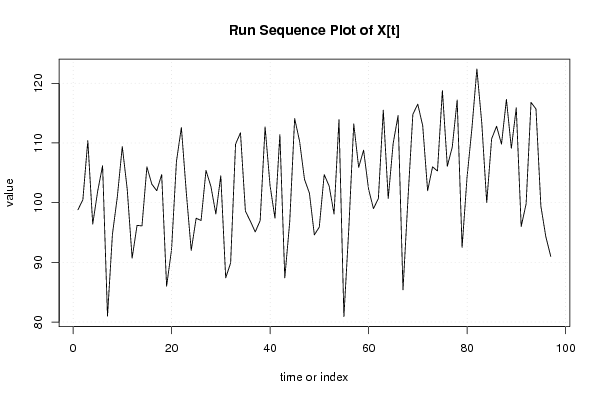
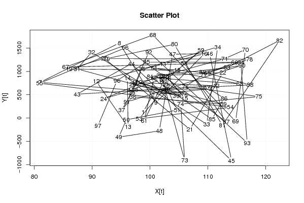
98.8 100.5 110.4 96.4 101.9 106.2 81 94.7 101 109.4 102.3 90.7 96.2 96.1 106 103.1 102 104.7 86 92.1 106.9 112.6 101.7 92 97.4 97 105.4 102.7 98.1 104.5 87.4 89.9 109.8 111.7 98.6 96.9 95.1 97 112.7 102.9 97.4 111.4 87.4 96.8 114.1 110.3 103.9 101.6 94.6 95.9 104.7 102.8 98.1 113.9 80.9 95.7 113.2 105.9 108.8 102.3 99 100.7 115.5 100.7 109.9 114.6 85.4 100.5 114.8 116.5 112.9 102 106 105.3 118.8 106.1 109.3 117.2 92.5 104.2 112.5 122.4 113.3 100 110.7 112.8 109.8 117.3 109.1 115.9 96 99.8 116.8 115.7 99.4 94.3 91 | |||||||||||||||||||||||||||||||||||||||||||||||||||||||||||||||||
| Dataseries Y: | |||||||||||||||||||||||||||||||||||||||||||||||||||||||||||||||||
128 502 629.7 595.9 823.7 498.7 766.9 1611.3 329.7 1378.9 1159.4 790.1 -189.6 862.4 426.6 852 834.7 1026.7 1052.8 1280.9 -243.6 976 908.2 416 610.7 728 520.8 905.8 768.9 479.3 1054.2 1411.9 -131 1526.2 1049.5 550.8 168.5 458.2 297 616.3 762.7 693.1 512.7 1169.2 -915.1 1384.2 1368.9 -275.1 -408.9 -37.5 171.5 671.8 -18.5 231.6 747.5 1505.7 -83.6 1173.2 1452.1 777 -52.8 861.2 735.2 1073.6 966.9 1189.8 1093.5 1782.7 -70.4 1471.6 1273.8 900.8 -910.2 299.8 460.2 677.2 937.1 1265.4 1275.6 1582.6 -154.2 1667.7 1083.1 891.7 -26.5 423.4 662.8 711.4 993.3 1133.2 343.9 1415.8 -531.8 1193.6 1201.3 805.6 -164.8 | |||||||||||||||||||||||||||||||||||||||||||||||||||||||||||||||||
Tables (Output of Computation) | |||||||||||||||||||||||||||||||||||||||||||||||||||||||||||||||||
| |||||||||||||||||||||||||||||||||||||||||||||||||||||||||||||||||
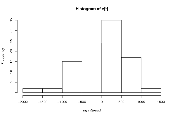
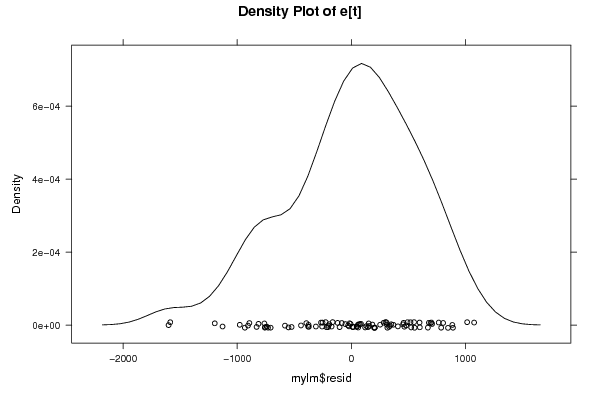
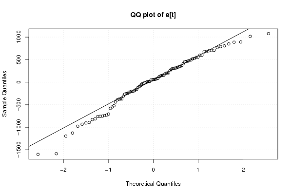
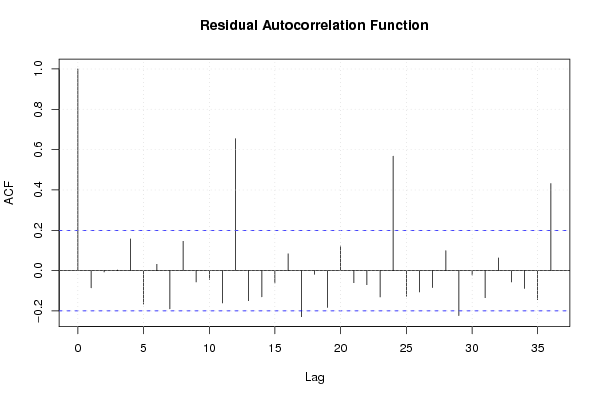
Figures (Output of Computation) | |||||||||||||||||||||||||||||||||||||||||||||||||||||||||||||||||
Input Parameters & R Code | |||||||||||||||||||||||||||||||||||||||||||||||||||||||||||||||||
| Parameters (Session): | |||||||||||||||||||||||||||||||||||||||||||||||||||||||||||||||||
| par1 = 0 ; par2 = 36 ; | |||||||||||||||||||||||||||||||||||||||||||||||||||||||||||||||||
| Parameters (R input): | |||||||||||||||||||||||||||||||||||||||||||||||||||||||||||||||||
| par1 = 0 ; par2 = 36 ; | |||||||||||||||||||||||||||||||||||||||||||||||||||||||||||||||||
| R code (references can be found in the software module): | |||||||||||||||||||||||||||||||||||||||||||||||||||||||||||||||||
par1 <- as.numeric(par1) | |||||||||||||||||||||||||||||||||||||||||||||||||||||||||||||||||