Repository of Reproducible Computations

Free Statistics

of Irreproducible Research!

Author's title

Author

*Unverified author*

R Software Module

rwasp_autocorrelation.wasp

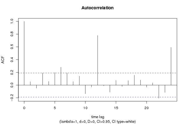
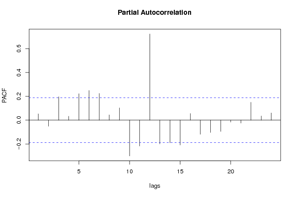
Title produced by software

(Partial) Autocorrelation Function

Date of computation

Tue, 15 Dec 2009 14:20:50 -0700

Cite this page as follows

Statistical Computations at FreeStatistics.org, Office for Research Development and Education, URL https://freestatistics.org/blog/index.php?v=date/2009/Dec/15/t1260912150q3yw2bb46ce6225.htm/, Retrieved Wed, 08 May 2024 22:18:58 +0000

Statistical Computations at FreeStatistics.org, Office for Research Development and Education, URL https://freestatistics.org/blog/index.php?pk=68178, Retrieved Wed, 08 May 2024 22:18:58 +0000

QR Codes:

Paste this QR Code to cite your computation.

Original text written by user:

IsPrivate?

No (this computation is public)

User-defined keywords

KDGP2W21

Estimated Impact

132

Family? (F = Feedback message, R = changed R code, M = changed R Module, P = changed Parameters, D = changed Data)

-       [(Partial) Autocorrelation Function] [] [2009-12-15 21:20:50] [ab5cffebaafedfca74d2c063d2ba2ba4] [Current]
- R  D    [(Partial) Autocorrelation Function] [] [2011-04-12 13:40:53] [81cdd92b187c11fcf96d69ee16e5a9b7] 

Feedback Forum

Post a new message

Dataseries X:

Download CSV

Histogram

Boxplots

Summary of computational transaction
Raw Input	view raw input (R code)
Raw Output	view raw output of R engine
Computing time	1 seconds
R Server	'Gwilym Jenkins' @ 72.249.127.135

\begin{tabular}{lllllllll}
\hline
Summary of computational transaction \tabularnewline
Raw Input & view raw input (R code)  \tabularnewline
Raw Output & view raw output of R engine  \tabularnewline
Computing time & 1 seconds \tabularnewline
R Server & 'Gwilym Jenkins' @ 72.249.127.135 \tabularnewline
\hline
\end{tabular}
%Source: https://freestatistics.org/blog/index.php?pk=68178&T=0

[TABLE]
[ROW][C]Summary of computational transaction[/C][/ROW]
[ROW][C]Raw Input[/C][C]view raw input (R code) [/C][/ROW]
[ROW][C]Raw Output[/C][C]view raw output of R engine [/C][/ROW]
[ROW][C]Computing time[/C][C]1 seconds[/C][/ROW]
[ROW][C]R Server[/C][C]'Gwilym Jenkins' @ 72.249.127.135[/C][/ROW]
[/TABLE]
Source: https://freestatistics.org/blog/index.php?pk=68178&T=0

Globally Unique Identifier (entire table): ba.freestatistics.org/blog/index.php?pk=68178&T=0

As an alternative you can also use a QR Code:

The GUIDs for individual cells are displayed in the table below:

Summary of computational transaction
Raw Input	view raw input (R code)
Raw Output	view raw output of R engine
Computing time	1 seconds
R Server	'Gwilym Jenkins' @ 72.249.127.135

Autocorrelation Function
Time lag k	ACF(k)	T-STAT	P-value
1	0.053018	0.551	0.291391
2	-0.048189	-0.5008	0.308769
3	0.190179	1.9764	0.025329
4	0.057118	0.5936	0.277014
5	0.19658	2.0429	0.021748
6	0.280837	2.9185	0.00214
7	0.189405	1.9684	0.025795
8	0.054652	0.568	0.285622
9	0.141014	1.4655	0.072851
10	-0.136409	-1.4176	0.079593
11	-0.031196	-0.3242	0.373209
12	0.778604	8.0915	0
13	-0.009886	-0.1027	0.459179
14	-0.111573	-1.1595	0.124406
15	0.072587	0.7543	0.226142
16	-0.023002	-0.239	0.405761
17	0.070302	0.7306	0.233303
18	0.155111	1.612	0.054944
19	0.079381	0.8249	0.20561
20	-0.03321	-0.3451	0.365335
21	0.035161	0.3654	0.357763
22	-0.205713	-2.1378	0.017393
23	-0.116541	-1.2111	0.114246
24	0.592363	6.156	0

\begin{tabular}{lllllllll}
\hline
Autocorrelation Function \tabularnewline
Time lag k & ACF(k) & T-STAT & P-value \tabularnewline
1 & 0.053018 & 0.551 & 0.291391 \tabularnewline
2 & -0.048189 & -0.5008 & 0.308769 \tabularnewline
3 & 0.190179 & 1.9764 & 0.025329 \tabularnewline
4 & 0.057118 & 0.5936 & 0.277014 \tabularnewline
5 & 0.19658 & 2.0429 & 0.021748 \tabularnewline
6 & 0.280837 & 2.9185 & 0.00214 \tabularnewline
7 & 0.189405 & 1.9684 & 0.025795 \tabularnewline
8 & 0.054652 & 0.568 & 0.285622 \tabularnewline
9 & 0.141014 & 1.4655 & 0.072851 \tabularnewline
10 & -0.136409 & -1.4176 & 0.079593 \tabularnewline
11 & -0.031196 & -0.3242 & 0.373209 \tabularnewline
12 & 0.778604 & 8.0915 & 0 \tabularnewline
13 & -0.009886 & -0.1027 & 0.459179 \tabularnewline
14 & -0.111573 & -1.1595 & 0.124406 \tabularnewline
15 & 0.072587 & 0.7543 & 0.226142 \tabularnewline
16 & -0.023002 & -0.239 & 0.405761 \tabularnewline
17 & 0.070302 & 0.7306 & 0.233303 \tabularnewline
18 & 0.155111 & 1.612 & 0.054944 \tabularnewline
19 & 0.079381 & 0.8249 & 0.20561 \tabularnewline
20 & -0.03321 & -0.3451 & 0.365335 \tabularnewline
21 & 0.035161 & 0.3654 & 0.357763 \tabularnewline
22 & -0.205713 & -2.1378 & 0.017393 \tabularnewline
23 & -0.116541 & -1.2111 & 0.114246 \tabularnewline
24 & 0.592363 & 6.156 & 0 \tabularnewline
\hline
\end{tabular}
%Source: https://freestatistics.org/blog/index.php?pk=68178&T=1

[TABLE]
[ROW][C]Autocorrelation Function[/C][/ROW]
[ROW][C]Time lag k[/C][C]ACF(k)[/C][C]T-STAT[/C][C]P-value[/C][/ROW]
[ROW][C]1[/C][C]0.053018[/C][C]0.551[/C][C]0.291391[/C][/ROW]
[ROW][C]2[/C][C]-0.048189[/C][C]-0.5008[/C][C]0.308769[/C][/ROW]
[ROW][C]3[/C][C]0.190179[/C][C]1.9764[/C][C]0.025329[/C][/ROW]
[ROW][C]4[/C][C]0.057118[/C][C]0.5936[/C][C]0.277014[/C][/ROW]
[ROW][C]5[/C][C]0.19658[/C][C]2.0429[/C][C]0.021748[/C][/ROW]
[ROW][C]6[/C][C]0.280837[/C][C]2.9185[/C][C]0.00214[/C][/ROW]
[ROW][C]7[/C][C]0.189405[/C][C]1.9684[/C][C]0.025795[/C][/ROW]
[ROW][C]8[/C][C]0.054652[/C][C]0.568[/C][C]0.285622[/C][/ROW]
[ROW][C]9[/C][C]0.141014[/C][C]1.4655[/C][C]0.072851[/C][/ROW]
[ROW][C]10[/C][C]-0.136409[/C][C]-1.4176[/C][C]0.079593[/C][/ROW]
[ROW][C]11[/C][C]-0.031196[/C][C]-0.3242[/C][C]0.373209[/C][/ROW]
[ROW][C]12[/C][C]0.778604[/C][C]8.0915[/C][C]0[/C][/ROW]
[ROW][C]13[/C][C]-0.009886[/C][C]-0.1027[/C][C]0.459179[/C][/ROW]
[ROW][C]14[/C][C]-0.111573[/C][C]-1.1595[/C][C]0.124406[/C][/ROW]
[ROW][C]15[/C][C]0.072587[/C][C]0.7543[/C][C]0.226142[/C][/ROW]
[ROW][C]16[/C][C]-0.023002[/C][C]-0.239[/C][C]0.405761[/C][/ROW]
[ROW][C]17[/C][C]0.070302[/C][C]0.7306[/C][C]0.233303[/C][/ROW]
[ROW][C]18[/C][C]0.155111[/C][C]1.612[/C][C]0.054944[/C][/ROW]
[ROW][C]19[/C][C]0.079381[/C][C]0.8249[/C][C]0.20561[/C][/ROW]
[ROW][C]20[/C][C]-0.03321[/C][C]-0.3451[/C][C]0.365335[/C][/ROW]
[ROW][C]21[/C][C]0.035161[/C][C]0.3654[/C][C]0.357763[/C][/ROW]
[ROW][C]22[/C][C]-0.205713[/C][C]-2.1378[/C][C]0.017393[/C][/ROW]
[ROW][C]23[/C][C]-0.116541[/C][C]-1.2111[/C][C]0.114246[/C][/ROW]
[ROW][C]24[/C][C]0.592363[/C][C]6.156[/C][C]0[/C][/ROW]
[/TABLE]
Source: https://freestatistics.org/blog/index.php?pk=68178&T=1

Globally Unique Identifier (entire table): ba.freestatistics.org/blog/index.php?pk=68178&T=1

As an alternative you can also use a QR Code:

The GUIDs for individual cells are displayed in the table below:

Autocorrelation Function
Time lag k	ACF(k)	T-STAT	P-value
1	0.053018	0.551	0.291391
2	-0.048189	-0.5008	0.308769
3	0.190179	1.9764	0.025329
4	0.057118	0.5936	0.277014
5	0.19658	2.0429	0.021748
6	0.280837	2.9185	0.00214
7	0.189405	1.9684	0.025795
8	0.054652	0.568	0.285622
9	0.141014	1.4655	0.072851
10	-0.136409	-1.4176	0.079593
11	-0.031196	-0.3242	0.373209
12	0.778604	8.0915	0
13	-0.009886	-0.1027	0.459179
14	-0.111573	-1.1595	0.124406
15	0.072587	0.7543	0.226142
16	-0.023002	-0.239	0.405761
17	0.070302	0.7306	0.233303
18	0.155111	1.612	0.054944
19	0.079381	0.8249	0.20561
20	-0.03321	-0.3451	0.365335
21	0.035161	0.3654	0.357763
22	-0.205713	-2.1378	0.017393
23	-0.116541	-1.2111	0.114246
24	0.592363	6.156	0

Partial Autocorrelation Function
Time lag k	PACF(k)	T-STAT	P-value
1	0.053018	0.551	0.291391
2	-0.051143	-0.5315	0.298083
3	0.196642	2.0436	0.021715
4	0.03262	0.339	0.367636
5	0.222234	2.3095	0.011408
6	0.249045	2.5882	0.005488
7	0.224214	2.3301	0.01083
8	0.044327	0.4607	0.322983
9	0.1029	1.0694	0.143643
10	-0.300738	-3.1254	0.001141
11	-0.217596	-2.2613	0.012871
12	0.723713	7.5211	0
13	-0.199544	-2.0737	0.020242
14	-0.190075	-1.9753	0.025392
15	-0.208923	-2.1712	0.016053
16	0.055884	0.5808	0.281304
17	-0.119096	-1.2377	0.109258
18	-0.103824	-1.079	0.141502
19	-0.094925	-0.9865	0.16305
20	-0.016339	-0.1698	0.432741
21	-0.024591	-0.2556	0.399389
22	0.149722	1.556	0.061322
23	0.035397	0.3679	0.356849
24	0.06041	0.6278	0.26573

\begin{tabular}{lllllllll}
\hline
Partial Autocorrelation Function \tabularnewline
Time lag k & PACF(k) & T-STAT & P-value \tabularnewline
1 & 0.053018 & 0.551 & 0.291391 \tabularnewline
2 & -0.051143 & -0.5315 & 0.298083 \tabularnewline
3 & 0.196642 & 2.0436 & 0.021715 \tabularnewline
4 & 0.03262 & 0.339 & 0.367636 \tabularnewline
5 & 0.222234 & 2.3095 & 0.011408 \tabularnewline
6 & 0.249045 & 2.5882 & 0.005488 \tabularnewline
7 & 0.224214 & 2.3301 & 0.01083 \tabularnewline
8 & 0.044327 & 0.4607 & 0.322983 \tabularnewline
9 & 0.1029 & 1.0694 & 0.143643 \tabularnewline
10 & -0.300738 & -3.1254 & 0.001141 \tabularnewline
11 & -0.217596 & -2.2613 & 0.012871 \tabularnewline
12 & 0.723713 & 7.5211 & 0 \tabularnewline
13 & -0.199544 & -2.0737 & 0.020242 \tabularnewline
14 & -0.190075 & -1.9753 & 0.025392 \tabularnewline
15 & -0.208923 & -2.1712 & 0.016053 \tabularnewline
16 & 0.055884 & 0.5808 & 0.281304 \tabularnewline
17 & -0.119096 & -1.2377 & 0.109258 \tabularnewline
18 & -0.103824 & -1.079 & 0.141502 \tabularnewline
19 & -0.094925 & -0.9865 & 0.16305 \tabularnewline
20 & -0.016339 & -0.1698 & 0.432741 \tabularnewline
21 & -0.024591 & -0.2556 & 0.399389 \tabularnewline
22 & 0.149722 & 1.556 & 0.061322 \tabularnewline
23 & 0.035397 & 0.3679 & 0.356849 \tabularnewline
24 & 0.06041 & 0.6278 & 0.26573 \tabularnewline
\hline
\end{tabular}
%Source: https://freestatistics.org/blog/index.php?pk=68178&T=2

[TABLE]
[ROW][C]Partial Autocorrelation Function[/C][/ROW]
[ROW][C]Time lag k[/C][C]PACF(k)[/C][C]T-STAT[/C][C]P-value[/C][/ROW]
[ROW][C]1[/C][C]0.053018[/C][C]0.551[/C][C]0.291391[/C][/ROW]
[ROW][C]2[/C][C]-0.051143[/C][C]-0.5315[/C][C]0.298083[/C][/ROW]
[ROW][C]3[/C][C]0.196642[/C][C]2.0436[/C][C]0.021715[/C][/ROW]
[ROW][C]4[/C][C]0.03262[/C][C]0.339[/C][C]0.367636[/C][/ROW]
[ROW][C]5[/C][C]0.222234[/C][C]2.3095[/C][C]0.011408[/C][/ROW]
[ROW][C]6[/C][C]0.249045[/C][C]2.5882[/C][C]0.005488[/C][/ROW]
[ROW][C]7[/C][C]0.224214[/C][C]2.3301[/C][C]0.01083[/C][/ROW]
[ROW][C]8[/C][C]0.044327[/C][C]0.4607[/C][C]0.322983[/C][/ROW]
[ROW][C]9[/C][C]0.1029[/C][C]1.0694[/C][C]0.143643[/C][/ROW]
[ROW][C]10[/C][C]-0.300738[/C][C]-3.1254[/C][C]0.001141[/C][/ROW]
[ROW][C]11[/C][C]-0.217596[/C][C]-2.2613[/C][C]0.012871[/C][/ROW]
[ROW][C]12[/C][C]0.723713[/C][C]7.5211[/C][C]0[/C][/ROW]
[ROW][C]13[/C][C]-0.199544[/C][C]-2.0737[/C][C]0.020242[/C][/ROW]
[ROW][C]14[/C][C]-0.190075[/C][C]-1.9753[/C][C]0.025392[/C][/ROW]
[ROW][C]15[/C][C]-0.208923[/C][C]-2.1712[/C][C]0.016053[/C][/ROW]
[ROW][C]16[/C][C]0.055884[/C][C]0.5808[/C][C]0.281304[/C][/ROW]
[ROW][C]17[/C][C]-0.119096[/C][C]-1.2377[/C][C]0.109258[/C][/ROW]
[ROW][C]18[/C][C]-0.103824[/C][C]-1.079[/C][C]0.141502[/C][/ROW]
[ROW][C]19[/C][C]-0.094925[/C][C]-0.9865[/C][C]0.16305[/C][/ROW]
[ROW][C]20[/C][C]-0.016339[/C][C]-0.1698[/C][C]0.432741[/C][/ROW]
[ROW][C]21[/C][C]-0.024591[/C][C]-0.2556[/C][C]0.399389[/C][/ROW]
[ROW][C]22[/C][C]0.149722[/C][C]1.556[/C][C]0.061322[/C][/ROW]
[ROW][C]23[/C][C]0.035397[/C][C]0.3679[/C][C]0.356849[/C][/ROW]
[ROW][C]24[/C][C]0.06041[/C][C]0.6278[/C][C]0.26573[/C][/ROW]
[/TABLE]
Source: https://freestatistics.org/blog/index.php?pk=68178&T=2

Globally Unique Identifier (entire table): ba.freestatistics.org/blog/index.php?pk=68178&T=2

As an alternative you can also use a QR Code:

The GUIDs for individual cells are displayed in the table below:

Partial Autocorrelation Function
Time lag k	PACF(k)	T-STAT	P-value
1	0.053018	0.551	0.291391
2	-0.051143	-0.5315	0.298083
3	0.196642	2.0436	0.021715
4	0.03262	0.339	0.367636
5	0.222234	2.3095	0.011408
6	0.249045	2.5882	0.005488
7	0.224214	2.3301	0.01083
8	0.044327	0.4607	0.322983
9	0.1029	1.0694	0.143643
10	-0.300738	-3.1254	0.001141
11	-0.217596	-2.2613	0.012871
12	0.723713	7.5211	0
13	-0.199544	-2.0737	0.020242
14	-0.190075	-1.9753	0.025392
15	-0.208923	-2.1712	0.016053
16	0.055884	0.5808	0.281304
17	-0.119096	-1.2377	0.109258
18	-0.103824	-1.079	0.141502
19	-0.094925	-0.9865	0.16305
20	-0.016339	-0.1698	0.432741
21	-0.024591	-0.2556	0.399389
22	0.149722	1.556	0.061322
23	0.035397	0.3679	0.356849
24	0.06041	0.6278	0.26573

Figure 1

PNG link

Postscript link

PDF link

Figure 2

PNG link

Postscript link

PDF link

Parameters (Session):

par1 = 24 ; par2 = 1 ; par3 = 0 ; par4 = 0 ; par5 = 12 ; par6 = White Noise ; par7 = 0.95 ;

Parameters (R input):

par1 = 24 ; par2 = 1 ; par3 = 0 ; par4 = 0 ; par5 = 12 ; par6 = White Noise ; par7 = 0.95 ;

R code (references can be found in the software module):

if (par1 == 'Default') {
par1 = 10*log10(length(x))
} else {
par1 <- as.numeric(par1)
}
par2 <- as.numeric(par2)
par3 <- as.numeric(par3)
par4 <- as.numeric(par4)
par5 <- as.numeric(par5)
if (par6 == 'White Noise') par6 <- 'white' else par6 <- 'ma'
par7 <- as.numeric(par7)
if (par2 == 0) {
x <- log(x)
} else {
x <- (x ^ par2 - 1) / par2
}
if (par3 > 0) x <- diff(x,lag=1,difference=par3)
if (par4 > 0) x <- diff(x,lag=par5,difference=par4)
bitmap(file='pic1.png')
racf <- acf(x, par1, main='Autocorrelation', xlab='time lag', ylab='ACF', ci.type=par6, ci=par7, sub=paste('(lambda=',par2,', d=',par3,', D=',par4,', CI=', par7, ', CI type=',par6,')',sep=''))
dev.off()
bitmap(file='pic2.png')
rpacf <- pacf(x,par1,main='Partial Autocorrelation',xlab='lags',ylab='PACF')
dev.off()
(myacf <- c(racf$acf))
(mypacf <- c(rpacf$acf))
lengthx <- length(x)
sqrtn <- sqrt(lengthx)
load(file='createtable')
a<-table.start()
a<-table.row.start(a)
a<-table.element(a,'Autocorrelation Function',4,TRUE)
a<-table.row.end(a)
a<-table.row.start(a)
a<-table.element(a,'Time lag k',header=TRUE)
a<-table.element(a,hyperlink('basics.htm','ACF(k)','click here for more information about the Autocorrelation Function'),header=TRUE)
a<-table.element(a,'T-STAT',header=TRUE)
a<-table.element(a,'P-value',header=TRUE)
a<-table.row.end(a)
for (i in 2:(par1+1)) {
a<-table.row.start(a)
a<-table.element(a,i-1,header=TRUE)
a<-table.element(a,round(myacf[i],6))
mytstat <- myacf[i]*sqrtn
a<-table.element(a,round(mytstat,4))
a<-table.element(a,round(1-pt(abs(mytstat),lengthx),6))
a<-table.row.end(a)
}
a<-table.end(a)
table.save(a,file='mytable.tab')
a<-table.start()
a<-table.row.start(a)
a<-table.element(a,'Partial Autocorrelation Function',4,TRUE)
a<-table.row.end(a)
a<-table.row.start(a)
a<-table.element(a,'Time lag k',header=TRUE)
a<-table.element(a,hyperlink('basics.htm','PACF(k)','click here for more information about the Partial Autocorrelation Function'),header=TRUE)
a<-table.element(a,'T-STAT',header=TRUE)
a<-table.element(a,'P-value',header=TRUE)
a<-table.row.end(a)
for (i in 1:par1) {
a<-table.row.start(a)
a<-table.element(a,i,header=TRUE)
a<-table.element(a,round(mypacf[i],6))
mytstat <- mypacf[i]*sqrtn
a<-table.element(a,round(mytstat,4))
a<-table.element(a,round(1-pt(abs(mytstat),lengthx),6))
a<-table.row.end(a)
}
a<-table.end(a)
table.save(a,file='mytable1.tab')

Free Statistics

Description of Statistical Computation

Tree of Dependent Computations

Dataset

Tables (Output of Computation)

Figures (Output of Computation)

Input Parameters & R Code