Repository of Reproducible Computations

Free Statistics

of Irreproducible Research!

Author's title

Author

*The author of this computation has been verified*

R Software Module

rwasp_boxcoxlin.wasp

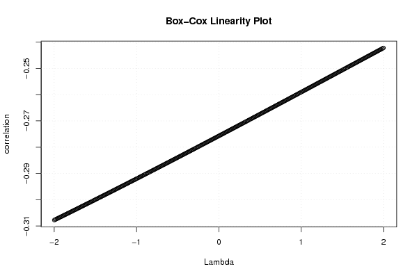
Title produced by software

Box-Cox Linearity Plot

Date of computation

Thu, 17 Dec 2009 02:38:35 -0700

Cite this page as follows

Statistical Computations at FreeStatistics.org, Office for Research Development and Education, URL https://freestatistics.org/blog/index.php?v=date/2009/Dec/17/t126104276416c3y5l91w3sz0j.htm/, Retrieved Tue, 30 Apr 2024 02:20:02 +0000

Statistical Computations at FreeStatistics.org, Office for Research Development and Education, URL https://freestatistics.org/blog/index.php?pk=68667, Retrieved Tue, 30 Apr 2024 02:20:02 +0000

QR Codes:

Paste this QR Code to cite your computation.

Original text written by user:

IsPrivate?

No (this computation is public)

User-defined keywords

x: W>25 y: Inflatie

Estimated Impact

157

Family? (F = Feedback message, R = changed R code, M = changed R Module, P = changed Parameters, D = changed Data)

-     [Partial Correlation] [CVM Paper: Partia...] [2009-12-17 09:09:51] [03d5b865e91ca35b5a5d21b8d6da5aba]
- RM D    [Box-Cox Linearity Plot] [CVM Paper: Box Co...] [2009-12-17 09:38:35] [a5ada8bd39e806b5b90f09589c89554a] [Current]

Feedback Forum

Post a new message

Dataseries X:

Download CSV

Histogram

Boxplots

7,5
7,4
7,1
6,8
6,9
7,2
7,4
7,3
6,9
6,9
6,8
7,1
7,2
7,1
7
6,9
7,1
7,3
7,5
7,5
7,5
7,3
7
6,7
6,5
6,5
6,5
6,6
6,8
6,9
6,9
6,8
6,8
6,5
6,1
6,1
5,9
5,7
5,9
5,9
6,1
6,3
6,2
5,9
5,7
5,4
5,6
6,2
6,3
6
5,6
5,5
5,9
6,5
6,8
6,8
6,5
6,2
6,2
6,5
6,7

Dataseries Y:

Download CSV

Histogram

2
1.8
2.7
2.3
1.9
2
2.3
2.8
2.4
2.3
2.7
2.7
2.9
3
2.2
2.3
2.8
2.8
2.8
2.2
2.6
2.8
2.5
2.4
2.3
1.9
1.7
2
2.1
1.7
1.8
1.8
1.8
1.3
1.3
1.3
1.2
1.4
2.2
2.9
3.1
3.5
3.6
4.4
4.1
5.1
5.8
5.9
5.4
5.5
4.8
3.2
2.7
2.1
1.9
0.6
0.7
-0.2
-1
-1.7
-0.7

Summary of computational transaction
Raw Input	view raw input (R code)
Raw Output	view raw output of R engine
Computing time	3 seconds
R Server	'Gwilym Jenkins' @ 72.249.127.135

\begin{tabular}{lllllllll}
\hline
Summary of computational transaction \tabularnewline
Raw Input & view raw input (R code)  \tabularnewline
Raw Output & view raw output of R engine  \tabularnewline
Computing time & 3 seconds \tabularnewline
R Server & 'Gwilym Jenkins' @ 72.249.127.135 \tabularnewline
\hline
\end{tabular}
%Source: https://freestatistics.org/blog/index.php?pk=68667&T=0

[TABLE]
[ROW][C]Summary of computational transaction[/C][/ROW]
[ROW][C]Raw Input[/C][C]view raw input (R code) [/C][/ROW]
[ROW][C]Raw Output[/C][C]view raw output of R engine [/C][/ROW]
[ROW][C]Computing time[/C][C]3 seconds[/C][/ROW]
[ROW][C]R Server[/C][C]'Gwilym Jenkins' @ 72.249.127.135[/C][/ROW]
[/TABLE]
Source: https://freestatistics.org/blog/index.php?pk=68667&T=0

Globally Unique Identifier (entire table): ba.freestatistics.org/blog/index.php?pk=68667&T=0

As an alternative you can also use a QR Code:

The GUIDs for individual cells are displayed in the table below:

Summary of computational transaction
Raw Input	view raw input (R code)
Raw Output	view raw output of R engine
Computing time	3 seconds
R Server	'Gwilym Jenkins' @ 72.249.127.135

Box-Cox Linearity Plot
# observations x	61
maximum correlation	0.307735981906645
optimal lambda(x)	-2
Residual SD (orginial)	1.41704554858837
Residual SD (transformed)	1.39593441847007

\begin{tabular}{lllllllll}
\hline
Box-Cox Linearity Plot \tabularnewline
# observations x & 61 \tabularnewline
maximum correlation & 0.307735981906645 \tabularnewline
optimal lambda(x) & -2 \tabularnewline
Residual SD (orginial) & 1.41704554858837 \tabularnewline
Residual SD (transformed) & 1.39593441847007 \tabularnewline
\hline
\end{tabular}
%Source: https://freestatistics.org/blog/index.php?pk=68667&T=1

[TABLE]
[ROW][C]Box-Cox Linearity Plot[/C][/ROW]
[ROW][C]# observations x[/C][C]61[/C][/ROW]
[ROW][C]maximum correlation[/C][C]0.307735981906645[/C][/ROW]
[ROW][C]optimal lambda(x)[/C][C]-2[/C][/ROW]
[ROW][C]Residual SD (orginial)[/C][C]1.41704554858837[/C][/ROW]
[ROW][C]Residual SD (transformed)[/C][C]1.39593441847007[/C][/ROW]
[/TABLE]
Source: https://freestatistics.org/blog/index.php?pk=68667&T=1

Globally Unique Identifier (entire table): ba.freestatistics.org/blog/index.php?pk=68667&T=1

As an alternative you can also use a QR Code:

The GUIDs for individual cells are displayed in the table below:

Box-Cox Linearity Plot
# observations x	61
maximum correlation	0.307735981906645
optimal lambda(x)	-2
Residual SD (orginial)	1.41704554858837
Residual SD (transformed)	1.39593441847007

Figure 1

PNG link

Postscript link

PDF link

Figure 2

PNG link

Postscript link

PDF link

Figure 3

PNG link

Postscript link

PDF link

Parameters (Session):

Parameters (R input):

R code (references can be found in the software module):

n <- length(x)
c <- array(NA,dim=c(401))
l <- array(NA,dim=c(401))
mx <- 0
mxli <- -999
for (i in 1:401)
{
l[i] <- (i-201)/100
if (l[i] != 0)
{
x1 <- (x^l[i] - 1) / l[i]
} else {
x1 <- log(x)
}
c[i] <- cor(x1,y)
if (mx < abs(c[i]))
{
mx <- abs(c[i])
mxli <- l[i]
}
}
c
mx
mxli
if (mxli != 0)
{
x1 <- (x^mxli - 1) / mxli
} else {
x1 <- log(x)
}
r<-lm(y~x)
se <- sqrt(var(r$residuals))
r1 <- lm(y~x1)
se1 <- sqrt(var(r1$residuals))
bitmap(file='test1.png')
plot(l,c,main='Box-Cox Linearity Plot',xlab='Lambda',ylab='correlation')
grid()
dev.off()
bitmap(file='test2.png')
plot(x,y,main='Linear Fit of Original Data',xlab='x',ylab='y')
abline(r)
grid()
mtext(paste('Residual Standard Deviation = ',se))
dev.off()
bitmap(file='test3.png')
plot(x1,y,main='Linear Fit of Transformed Data',xlab='x',ylab='y')
abline(r1)
grid()
mtext(paste('Residual Standard Deviation = ',se1))
dev.off()
load(file='createtable')
a<-table.start()
a<-table.row.start(a)
a<-table.element(a,'Box-Cox Linearity Plot',2,TRUE)
a<-table.row.end(a)
a<-table.row.start(a)
a<-table.element(a,'# observations x',header=TRUE)
a<-table.element(a,n)
a<-table.row.end(a)
a<-table.row.start(a)
a<-table.element(a,'maximum correlation',header=TRUE)
a<-table.element(a,mx)
a<-table.row.end(a)
a<-table.row.start(a)
a<-table.element(a,'optimal lambda(x)',header=TRUE)
a<-table.element(a,mxli)
a<-table.row.end(a)
a<-table.row.start(a)
a<-table.element(a,'Residual SD (orginial)',header=TRUE)
a<-table.element(a,se)
a<-table.row.end(a)
a<-table.row.start(a)
a<-table.element(a,'Residual SD (transformed)',header=TRUE)
a<-table.element(a,se1)
a<-table.row.end(a)
a<-table.end(a)
table.save(a,file='mytable.tab')

Free Statistics

Description of Statistical Computation

Tree of Dependent Computations

Dataset

Tables (Output of Computation)

Figures (Output of Computation)

Input Parameters & R Code