Free Statistics
of Irreproducible Research!
Description of Statistical Computation | |||||||||||||||||||||||||||||||||||||||||||||||||||||||||||||||||
|---|---|---|---|---|---|---|---|---|---|---|---|---|---|---|---|---|---|---|---|---|---|---|---|---|---|---|---|---|---|---|---|---|---|---|---|---|---|---|---|---|---|---|---|---|---|---|---|---|---|---|---|---|---|---|---|---|---|---|---|---|---|---|---|---|---|
| Author's title | |||||||||||||||||||||||||||||||||||||||||||||||||||||||||||||||||
| Author | *The author of this computation has been verified* | ||||||||||||||||||||||||||||||||||||||||||||||||||||||||||||||||
| R Software Module | rwasp_edabi.wasp | ||||||||||||||||||||||||||||||||||||||||||||||||||||||||||||||||
| Title produced by software | Bivariate Explorative Data Analysis | ||||||||||||||||||||||||||||||||||||||||||||||||||||||||||||||||
| Date of computation | Thu, 17 Dec 2009 02:40:23 -0700 | ||||||||||||||||||||||||||||||||||||||||||||||||||||||||||||||||
| Cite this page as follows | Statistical Computations at FreeStatistics.org, Office for Research Development and Education, URL https://freestatistics.org/blog/index.php?v=date/2009/Dec/17/t126104287111fj3fm96acvv24.htm/, Retrieved Tue, 30 Apr 2024 06:40:49 +0000 | ||||||||||||||||||||||||||||||||||||||||||||||||||||||||||||||||
| Statistical Computations at FreeStatistics.org, Office for Research Development and Education, URL https://freestatistics.org/blog/index.php?pk=68668, Retrieved Tue, 30 Apr 2024 06:40:49 +0000 | |||||||||||||||||||||||||||||||||||||||||||||||||||||||||||||||||
| QR Codes: | |||||||||||||||||||||||||||||||||||||||||||||||||||||||||||||||||
|
| |||||||||||||||||||||||||||||||||||||||||||||||||||||||||||||||||
| Original text written by user: | |||||||||||||||||||||||||||||||||||||||||||||||||||||||||||||||||
| IsPrivate? | No (this computation is public) | ||||||||||||||||||||||||||||||||||||||||||||||||||||||||||||||||
| User-defined keywords | SHW Paper: Bivariate EDA | ||||||||||||||||||||||||||||||||||||||||||||||||||||||||||||||||
| Estimated Impact | 166 | ||||||||||||||||||||||||||||||||||||||||||||||||||||||||||||||||
Tree of Dependent Computations | |||||||||||||||||||||||||||||||||||||||||||||||||||||||||||||||||
| Family? (F = Feedback message, R = changed R code, M = changed R Module, P = changed Parameters, D = changed Data) | |||||||||||||||||||||||||||||||||||||||||||||||||||||||||||||||||
| - [Bivariate Data Series] [Bivariate dataset] [2008-01-05 23:51:08] [74be16979710d4c4e7c6647856088456] - RMPD [Bivariate Explorative Data Analysis] [WS 4 - Deel 1 - V...] [2009-10-26 08:28:42] [b103a1dc147def8132c7f643ad8c8f84] - M D [Bivariate Explorative Data Analysis] [Paper: Bivariate EDA] [2009-12-17 09:40:23] [a45cc820faa25ce30779915639528ec2] [Current] - D [Bivariate Explorative Data Analysis] [Paper Bivariate E...] [2009-12-17 13:23:43] [4395c69e961f9a13a0559fd2f0a72538] - RMPD [Central Tendency] [Paper Robustness ...] [2009-12-17 13:29:44] [4395c69e961f9a13a0559fd2f0a72538] - RMP [Bivariate Kernel Density Estimation] [Paper Bivariate K...] [2009-12-17 13:34:57] [4395c69e961f9a13a0559fd2f0a72538] - RMP [Pearson Correlation] [Paper Pearson Cor...] [2009-12-17 13:40:11] [4395c69e961f9a13a0559fd2f0a72538] | |||||||||||||||||||||||||||||||||||||||||||||||||||||||||||||||||
| Feedback Forum | |||||||||||||||||||||||||||||||||||||||||||||||||||||||||||||||||
Post a new message | |||||||||||||||||||||||||||||||||||||||||||||||||||||||||||||||||
Dataset | |||||||||||||||||||||||||||||||||||||||||||||||||||||||||||||||||
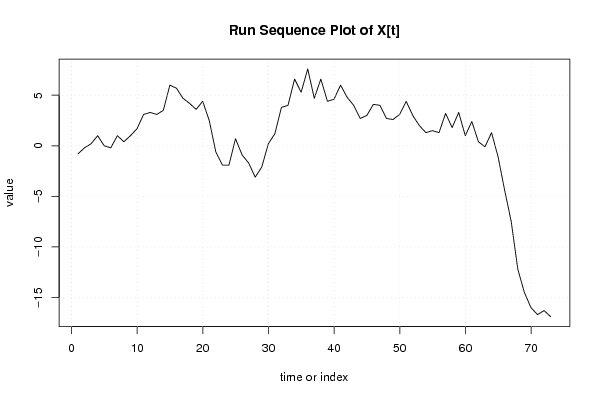
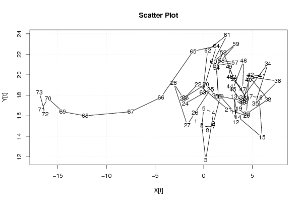
| Dataseries X: | |||||||||||||||||||||||||||||||||||||||||||||||||||||||||||||||||
-0.8 -0.2 0.2 1 0 -0.2 1 0.4 1 1.7 3.1 3.3 3.1 3.5 6 5.7 4.7 4.2 3.6 4.4 2.5 -0.6 -1.9 -1.9 0.7 -0.9 -1.7 -3.1 -2.1 0.2 1.2 3.8 4 6.6 5.3 7.6 4.7 6.6 4.4 4.6 6 4.8 4 2.7 3 4.1 4 2.7 2.6 3.1 4.4 3 2 1.3 1.5 1.3 3.2 1.8 3.3 1 2.4 0.4 -0.1 1.3 -1.1 -4.4 -7.5 -12.2 -14.5 -16 -16.7 -16.3 -16.9 | |||||||||||||||||||||||||||||||||||||||||||||||||||||||||||||||||
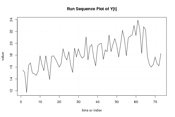
| Dataseries Y: | |||||||||||||||||||||||||||||||||||||||||||||||||||||||||||||||||
15,5 15,1 11,7 16,3 16,7 15 14,9 14,6 15,3 17,9 16,4 15,4 17,9 15,9 13,9 17,8 17,9 17,4 16,7 16 16,6 19,1 17,8 17,2 18,6 16,3 15,1 19,2 17,7 19,1 18 17,5 17,8 21,1 17,2 19,4 19,8 17,6 16,2 19,5 19,9 20 17,3 18,9 18,6 21,4 18,6 19,8 20,8 19,6 17,7 19,8 22,2 20,7 17,9 20,9 21,2 21,4 23 21,3 23,9 22,4 18,3 22,8 22,3 17,8 16,4 16 16,4 17,7 16,6 16,2 18,3 | |||||||||||||||||||||||||||||||||||||||||||||||||||||||||||||||||
Tables (Output of Computation) | |||||||||||||||||||||||||||||||||||||||||||||||||||||||||||||||||
| |||||||||||||||||||||||||||||||||||||||||||||||||||||||||||||||||
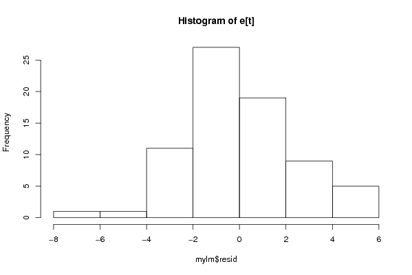
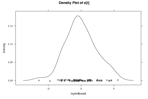
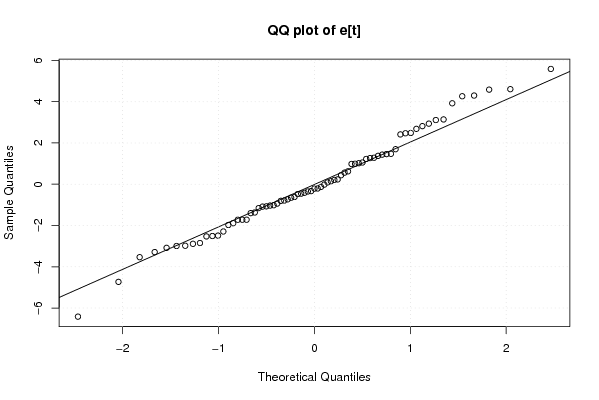
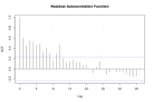
Figures (Output of Computation) | |||||||||||||||||||||||||||||||||||||||||||||||||||||||||||||||||
Input Parameters & R Code | |||||||||||||||||||||||||||||||||||||||||||||||||||||||||||||||||
| Parameters (Session): | |||||||||||||||||||||||||||||||||||||||||||||||||||||||||||||||||
| par1 = 0 ; par2 = 36 ; | |||||||||||||||||||||||||||||||||||||||||||||||||||||||||||||||||
| Parameters (R input): | |||||||||||||||||||||||||||||||||||||||||||||||||||||||||||||||||
| par1 = 0 ; par2 = 36 ; | |||||||||||||||||||||||||||||||||||||||||||||||||||||||||||||||||
| R code (references can be found in the software module): | |||||||||||||||||||||||||||||||||||||||||||||||||||||||||||||||||
par1 <- as.numeric(par1) | |||||||||||||||||||||||||||||||||||||||||||||||||||||||||||||||||