Free Statistics
of Irreproducible Research!
Description of Statistical Computation | |||||||||||||||||||||
|---|---|---|---|---|---|---|---|---|---|---|---|---|---|---|---|---|---|---|---|---|---|
| Author's title | |||||||||||||||||||||
| Author | *The author of this computation has been verified* | ||||||||||||||||||||
| R Software Module | rwasp_cloud.wasp | ||||||||||||||||||||
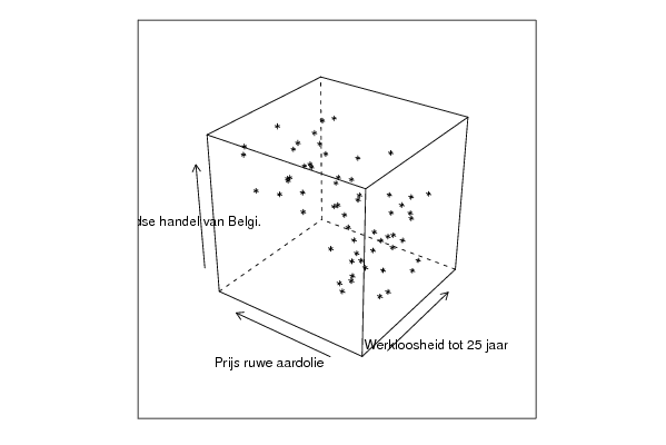
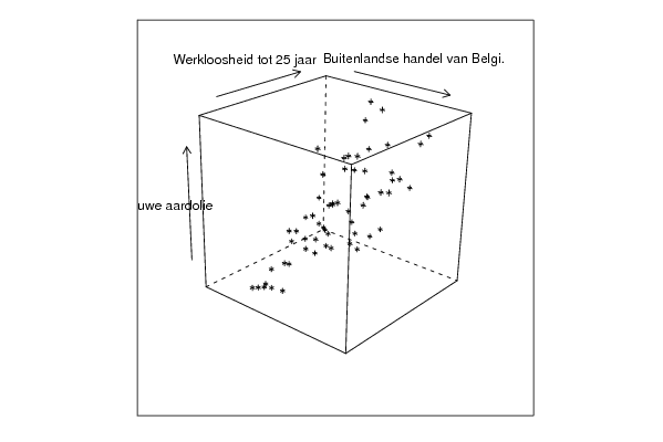
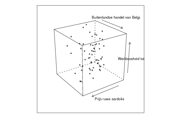
| Title produced by software | Trivariate Scatterplots | ||||||||||||||||||||
| Date of computation | Thu, 17 Dec 2009 04:10:11 -0700 | ||||||||||||||||||||
| Cite this page as follows | Statistical Computations at FreeStatistics.org, Office for Research Development and Education, URL https://freestatistics.org/blog/index.php?v=date/2009/Dec/17/t12610491162ieqspub23ks6tq.htm/, Retrieved Tue, 30 Apr 2024 01:26:23 +0000 | ||||||||||||||||||||
| Statistical Computations at FreeStatistics.org, Office for Research Development and Education, URL https://freestatistics.org/blog/index.php?pk=68758, Retrieved Tue, 30 Apr 2024 01:26:23 +0000 | |||||||||||||||||||||
| QR Codes: | |||||||||||||||||||||
|
| |||||||||||||||||||||
| Original text written by user: | |||||||||||||||||||||
| IsPrivate? | No (this computation is public) | ||||||||||||||||||||
| User-defined keywords | |||||||||||||||||||||
| Estimated Impact | 197 | ||||||||||||||||||||
Tree of Dependent Computations | |||||||||||||||||||||
| Family? (F = Feedback message, R = changed R code, M = changed R Module, P = changed Parameters, D = changed Data) | |||||||||||||||||||||
| - [Bivariate Data Series] [Bivariate dataset] [2008-01-05 23:51:08] [74be16979710d4c4e7c6647856088456] F RMPD [Univariate Explorative Data Analysis] [Colombia Coffee] [2008-01-07 14:21:11] [74be16979710d4c4e7c6647856088456] F RMPD [Univariate Data Series] [] [2009-10-14 08:30:28] [74be16979710d4c4e7c6647856088456] - RMPD [Partial Correlation] [Partial Correlation] [2009-12-16 14:03:17] [4d62210f0915d3a20cbf115865da7cd4] - D [Partial Correlation] [Partial Correlation] [2009-12-16 14:13:22] [4d62210f0915d3a20cbf115865da7cd4] - RMP [Trivariate Scatterplots] [Trivariate Scatte...] [2009-12-17 11:10:11] [91df150cd527c563f0151b3a845ecd72] [Current] - RMPD [Kendall tau Correlation Matrix] [Kendall tau corre...] [2009-12-18 15:21:58] [4d62210f0915d3a20cbf115865da7cd4] - P [Kendall tau Correlation Matrix] [Pearson Correlati...] [2010-12-14 18:53:01] [8214fe6d084e5ad7598b249a26cc9f06] | |||||||||||||||||||||
| Feedback Forum | |||||||||||||||||||||
Post a new message | |||||||||||||||||||||
Dataset | |||||||||||||||||||||
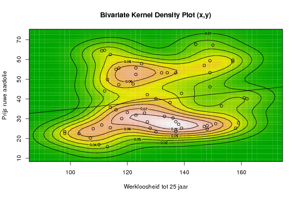
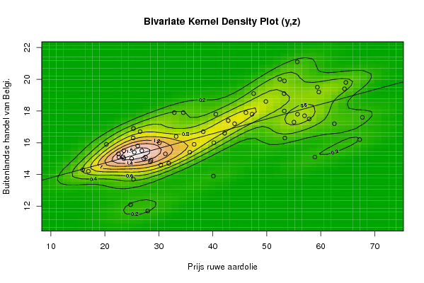
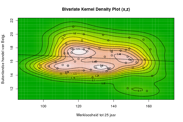
| Dataseries X: | |||||||||||||||||||||
113 110 107 103 98 98 137 148 147 139 130 128 127 123 118 114 108 111 151 159 158 148 138 137 136 133 126 120 114 116 153 162 161 149 139 135 130 127 122 117 112 113 149 157 157 147 137 132 125 123 117 114 111 112 144 150 149 134 123 116 | |||||||||||||||||||||
| Dataseries Y: | |||||||||||||||||||||
15.89 16.93 20.28 22.52 23.51 22.59 23.51 24.76 26.08 25.29 23.38 25.29 28.42 31.85 30.1 25.45 24.95 26.84 27.52 27.94 25.23 26.53 27.21 28.53 30.35 31.21 32.86 33.2 35.73 34.53 36.54 40.1 40.56 46.14 42.85 38.22 40.18 42.19 47.56 47.26 44.03 49.83 53.35 58.9 59.64 56.99 53.2 53.24 57.85 55.69 55.64 62.52 64.4 64.65 67.71 67.21 59.37 53.26 52.42 55.03 | |||||||||||||||||||||
| Dataseries Z: | |||||||||||||||||||||
14.3 14.2 15.9 15.3 15.5 15.1 15 12.1 15.8 16.9 15.1 13.7 14.8 14.7 16 15.4 15 15.5 15.1 11.7 16.3 16.7 15 14.9 14.6 15.3 17.9 16.4 15.4 17.9 15.9 13.9 17.8 17.9 17.4 16.7 16 16.6 19.1 17.8 17.2 18.6 16.3 15.1 19.2 17.7 19.1 18 17.5 17.8 21.1 17.2 19.4 19.8 17.6 16.2 19.5 19.9 20 17.3 | |||||||||||||||||||||
Tables (Output of Computation) | |||||||||||||||||||||
| |||||||||||||||||||||
Figures (Output of Computation) | |||||||||||||||||||||
Input Parameters & R Code | |||||||||||||||||||||
| Parameters (Session): | |||||||||||||||||||||
| par1 = 50 ; par2 = 50 ; par3 = Y ; par4 = Y ; par5 = Werkloosheid tot 25 jaar ; par6 = Prijs ruwe aardolie ; par7 = Buitenlandse handel van Belgi� ; | |||||||||||||||||||||
| Parameters (R input): | |||||||||||||||||||||
| par1 = 50 ; par2 = 50 ; par3 = Y ; par4 = Y ; par5 = Werkloosheid tot 25 jaar ; par6 = Prijs ruwe aardolie ; par7 = Buitenlandse handel van Belgi� ; | |||||||||||||||||||||
| R code (references can be found in the software module): | |||||||||||||||||||||
x <- array(x,dim=c(length(x),1)) | |||||||||||||||||||||