Repository of Reproducible Computations

Free Statistics

of Irreproducible Research!

Author's title

Author

*Unverified author*

R Software Module

rwasp_autocorrelation.wasp

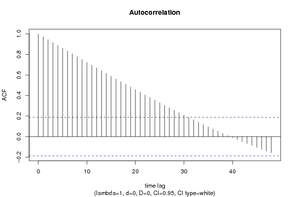
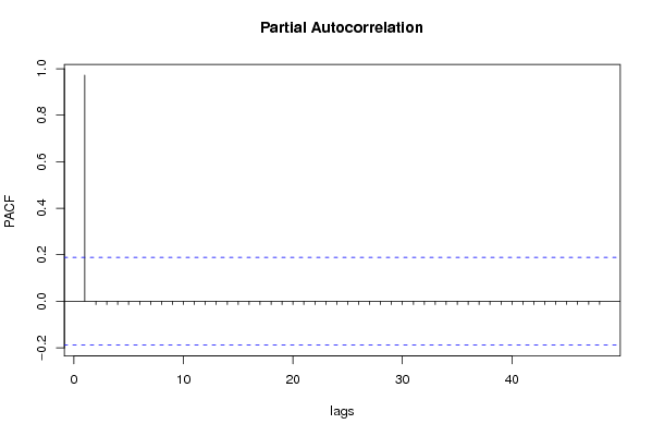
Title produced by software

(Partial) Autocorrelation Function

Date of computation

Thu, 17 Dec 2009 06:10:56 -0700

Cite this page as follows

Statistical Computations at FreeStatistics.org, Office for Research Development and Education, URL https://freestatistics.org/blog/index.php?v=date/2009/Dec/17/t1261055506iv3bd1jqs12s2fr.htm/, Retrieved Tue, 30 Apr 2024 03:34:00 +0000

Statistical Computations at FreeStatistics.org, Office for Research Development and Education, URL https://freestatistics.org/blog/index.php?pk=68847, Retrieved Tue, 30 Apr 2024 03:34:00 +0000

QR Codes:

Paste this QR Code to cite your computation.

Original text written by user:

IsPrivate?

No (this computation is public)

User-defined keywords

KDGP2W21

Estimated Impact

Family? (F = Feedback message, R = changed R code, M = changed R Module, P = changed Parameters, D = changed Data)

-       [(Partial) Autocorrelation Function] [Autocorrelatie bl...] [2009-12-17 13:10:56] [1596366c2ece8f787477cc7d1246d4c7] [Current]

Feedback Forum

Post a new message

Dataseries X:

Download CSV

Histogram

Boxplots

Summary of computational transaction
Raw Input	view raw input (R code)
Raw Output	view raw output of R engine
Computing time	1 seconds
R Server	'Gwilym Jenkins' @ 72.249.127.135

\begin{tabular}{lllllllll}
\hline
Summary of computational transaction \tabularnewline
Raw Input & view raw input (R code)  \tabularnewline
Raw Output & view raw output of R engine  \tabularnewline
Computing time & 1 seconds \tabularnewline
R Server & 'Gwilym Jenkins' @ 72.249.127.135 \tabularnewline
\hline
\end{tabular}
%Source: https://freestatistics.org/blog/index.php?pk=68847&T=0

[TABLE]
[ROW][C]Summary of computational transaction[/C][/ROW]
[ROW][C]Raw Input[/C][C]view raw input (R code) [/C][/ROW]
[ROW][C]Raw Output[/C][C]view raw output of R engine [/C][/ROW]
[ROW][C]Computing time[/C][C]1 seconds[/C][/ROW]
[ROW][C]R Server[/C][C]'Gwilym Jenkins' @ 72.249.127.135[/C][/ROW]
[/TABLE]
Source: https://freestatistics.org/blog/index.php?pk=68847&T=0

Globally Unique Identifier (entire table): ba.freestatistics.org/blog/index.php?pk=68847&T=0

As an alternative you can also use a QR Code:

The GUIDs for individual cells are displayed in the table below:

Summary of computational transaction
Raw Input	view raw input (R code)
Raw Output	view raw output of R engine
Computing time	1 seconds
R Server	'Gwilym Jenkins' @ 72.249.127.135

Autocorrelation Function
Time lag k	ACF(k)	T-STAT	P-value
1	0.972222	10.1036	0
2	0.944454	9.8151	0
3	0.916705	9.5267	0
4	0.888984	9.2386	0
5	0.861302	8.9509	0
6	0.833667	8.6637	0
7	0.806089	8.3771	0
8	0.778578	8.0912	0
9	0.751143	7.8061	0
10	0.723794	7.5219	0
11	0.69654	7.2387	0
12	0.669391	6.9565	0
13	0.642357	6.6756	0
14	0.615446	6.3959	0
15	0.588668	6.1176	0
16	0.562034	5.8408	0
17	0.535552	5.5656	0
18	0.509231	5.2921	0
19	0.483083	5.0203	1e-06
20	0.457115	4.7505	3e-06
21	0.431338	4.4826	9e-06
22	0.405761	4.2168	2.6e-05
23	0.380393	3.9532	6.9e-05
24	0.355245	3.6918	0.000175
25	0.330325	3.4328	0.000424
26	0.305644	3.1763	0.000972
27	0.28121	2.9224	0.002115
28	0.257033	2.6712	0.004364
29	0.233123	2.4227	0.008535
30	0.20949	2.1771	0.015826
31	0.186142	1.9344	0.027837
32	0.163089	1.6949	0.04649
33	0.140342	1.4585	0.073806
34	0.117908	1.2253	0.111556
35	0.095799	0.9956	0.160841
36	0.074023	0.7693	0.221705
37	0.05259	0.5465	0.292913
38	0.03151	0.3275	0.371977
39	0.010791	0.1121	0.455457
40	-0.009555	-0.0993	0.460541
41	-0.029521	-0.3068	0.379796
42	-0.049096	-0.5102	0.305468
43	-0.068271	-0.7095	0.239772
44	-0.087037	-0.9045	0.183868
45	-0.105383	-1.0952	0.137938
46	-0.123301	-1.2814	0.101403
47	-0.14078	-1.463	0.073182
48	-0.157812	-1.64	0.051955

\begin{tabular}{lllllllll}
\hline
Autocorrelation Function \tabularnewline
Time lag k & ACF(k) & T-STAT & P-value \tabularnewline
1 & 0.972222 & 10.1036 & 0 \tabularnewline
2 & 0.944454 & 9.8151 & 0 \tabularnewline
3 & 0.916705 & 9.5267 & 0 \tabularnewline
4 & 0.888984 & 9.2386 & 0 \tabularnewline
5 & 0.861302 & 8.9509 & 0 \tabularnewline
6 & 0.833667 & 8.6637 & 0 \tabularnewline
7 & 0.806089 & 8.3771 & 0 \tabularnewline
8 & 0.778578 & 8.0912 & 0 \tabularnewline
9 & 0.751143 & 7.8061 & 0 \tabularnewline
10 & 0.723794 & 7.5219 & 0 \tabularnewline
11 & 0.69654 & 7.2387 & 0 \tabularnewline
12 & 0.669391 & 6.9565 & 0 \tabularnewline
13 & 0.642357 & 6.6756 & 0 \tabularnewline
14 & 0.615446 & 6.3959 & 0 \tabularnewline
15 & 0.588668 & 6.1176 & 0 \tabularnewline
16 & 0.562034 & 5.8408 & 0 \tabularnewline
17 & 0.535552 & 5.5656 & 0 \tabularnewline
18 & 0.509231 & 5.2921 & 0 \tabularnewline
19 & 0.483083 & 5.0203 & 1e-06 \tabularnewline
20 & 0.457115 & 4.7505 & 3e-06 \tabularnewline
21 & 0.431338 & 4.4826 & 9e-06 \tabularnewline
22 & 0.405761 & 4.2168 & 2.6e-05 \tabularnewline
23 & 0.380393 & 3.9532 & 6.9e-05 \tabularnewline
24 & 0.355245 & 3.6918 & 0.000175 \tabularnewline
25 & 0.330325 & 3.4328 & 0.000424 \tabularnewline
26 & 0.305644 & 3.1763 & 0.000972 \tabularnewline
27 & 0.28121 & 2.9224 & 0.002115 \tabularnewline
28 & 0.257033 & 2.6712 & 0.004364 \tabularnewline
29 & 0.233123 & 2.4227 & 0.008535 \tabularnewline
30 & 0.20949 & 2.1771 & 0.015826 \tabularnewline
31 & 0.186142 & 1.9344 & 0.027837 \tabularnewline
32 & 0.163089 & 1.6949 & 0.04649 \tabularnewline
33 & 0.140342 & 1.4585 & 0.073806 \tabularnewline
34 & 0.117908 & 1.2253 & 0.111556 \tabularnewline
35 & 0.095799 & 0.9956 & 0.160841 \tabularnewline
36 & 0.074023 & 0.7693 & 0.221705 \tabularnewline
37 & 0.05259 & 0.5465 & 0.292913 \tabularnewline
38 & 0.03151 & 0.3275 & 0.371977 \tabularnewline
39 & 0.010791 & 0.1121 & 0.455457 \tabularnewline
40 & -0.009555 & -0.0993 & 0.460541 \tabularnewline
41 & -0.029521 & -0.3068 & 0.379796 \tabularnewline
42 & -0.049096 & -0.5102 & 0.305468 \tabularnewline
43 & -0.068271 & -0.7095 & 0.239772 \tabularnewline
44 & -0.087037 & -0.9045 & 0.183868 \tabularnewline
45 & -0.105383 & -1.0952 & 0.137938 \tabularnewline
46 & -0.123301 & -1.2814 & 0.101403 \tabularnewline
47 & -0.14078 & -1.463 & 0.073182 \tabularnewline
48 & -0.157812 & -1.64 & 0.051955 \tabularnewline
\hline
\end{tabular}
%Source: https://freestatistics.org/blog/index.php?pk=68847&T=1

[TABLE]
[ROW][C]Autocorrelation Function[/C][/ROW]
[ROW][C]Time lag k[/C][C]ACF(k)[/C][C]T-STAT[/C][C]P-value[/C][/ROW]
[ROW][C]1[/C][C]0.972222[/C][C]10.1036[/C][C]0[/C][/ROW]
[ROW][C]2[/C][C]0.944454[/C][C]9.8151[/C][C]0[/C][/ROW]
[ROW][C]3[/C][C]0.916705[/C][C]9.5267[/C][C]0[/C][/ROW]
[ROW][C]4[/C][C]0.888984[/C][C]9.2386[/C][C]0[/C][/ROW]
[ROW][C]5[/C][C]0.861302[/C][C]8.9509[/C][C]0[/C][/ROW]
[ROW][C]6[/C][C]0.833667[/C][C]8.6637[/C][C]0[/C][/ROW]
[ROW][C]7[/C][C]0.806089[/C][C]8.3771[/C][C]0[/C][/ROW]
[ROW][C]8[/C][C]0.778578[/C][C]8.0912[/C][C]0[/C][/ROW]
[ROW][C]9[/C][C]0.751143[/C][C]7.8061[/C][C]0[/C][/ROW]
[ROW][C]10[/C][C]0.723794[/C][C]7.5219[/C][C]0[/C][/ROW]
[ROW][C]11[/C][C]0.69654[/C][C]7.2387[/C][C]0[/C][/ROW]
[ROW][C]12[/C][C]0.669391[/C][C]6.9565[/C][C]0[/C][/ROW]
[ROW][C]13[/C][C]0.642357[/C][C]6.6756[/C][C]0[/C][/ROW]
[ROW][C]14[/C][C]0.615446[/C][C]6.3959[/C][C]0[/C][/ROW]
[ROW][C]15[/C][C]0.588668[/C][C]6.1176[/C][C]0[/C][/ROW]
[ROW][C]16[/C][C]0.562034[/C][C]5.8408[/C][C]0[/C][/ROW]
[ROW][C]17[/C][C]0.535552[/C][C]5.5656[/C][C]0[/C][/ROW]
[ROW][C]18[/C][C]0.509231[/C][C]5.2921[/C][C]0[/C][/ROW]
[ROW][C]19[/C][C]0.483083[/C][C]5.0203[/C][C]1e-06[/C][/ROW]
[ROW][C]20[/C][C]0.457115[/C][C]4.7505[/C][C]3e-06[/C][/ROW]
[ROW][C]21[/C][C]0.431338[/C][C]4.4826[/C][C]9e-06[/C][/ROW]
[ROW][C]22[/C][C]0.405761[/C][C]4.2168[/C][C]2.6e-05[/C][/ROW]
[ROW][C]23[/C][C]0.380393[/C][C]3.9532[/C][C]6.9e-05[/C][/ROW]
[ROW][C]24[/C][C]0.355245[/C][C]3.6918[/C][C]0.000175[/C][/ROW]
[ROW][C]25[/C][C]0.330325[/C][C]3.4328[/C][C]0.000424[/C][/ROW]
[ROW][C]26[/C][C]0.305644[/C][C]3.1763[/C][C]0.000972[/C][/ROW]
[ROW][C]27[/C][C]0.28121[/C][C]2.9224[/C][C]0.002115[/C][/ROW]
[ROW][C]28[/C][C]0.257033[/C][C]2.6712[/C][C]0.004364[/C][/ROW]
[ROW][C]29[/C][C]0.233123[/C][C]2.4227[/C][C]0.008535[/C][/ROW]
[ROW][C]30[/C][C]0.20949[/C][C]2.1771[/C][C]0.015826[/C][/ROW]
[ROW][C]31[/C][C]0.186142[/C][C]1.9344[/C][C]0.027837[/C][/ROW]
[ROW][C]32[/C][C]0.163089[/C][C]1.6949[/C][C]0.04649[/C][/ROW]
[ROW][C]33[/C][C]0.140342[/C][C]1.4585[/C][C]0.073806[/C][/ROW]
[ROW][C]34[/C][C]0.117908[/C][C]1.2253[/C][C]0.111556[/C][/ROW]
[ROW][C]35[/C][C]0.095799[/C][C]0.9956[/C][C]0.160841[/C][/ROW]
[ROW][C]36[/C][C]0.074023[/C][C]0.7693[/C][C]0.221705[/C][/ROW]
[ROW][C]37[/C][C]0.05259[/C][C]0.5465[/C][C]0.292913[/C][/ROW]
[ROW][C]38[/C][C]0.03151[/C][C]0.3275[/C][C]0.371977[/C][/ROW]
[ROW][C]39[/C][C]0.010791[/C][C]0.1121[/C][C]0.455457[/C][/ROW]
[ROW][C]40[/C][C]-0.009555[/C][C]-0.0993[/C][C]0.460541[/C][/ROW]
[ROW][C]41[/C][C]-0.029521[/C][C]-0.3068[/C][C]0.379796[/C][/ROW]
[ROW][C]42[/C][C]-0.049096[/C][C]-0.5102[/C][C]0.305468[/C][/ROW]
[ROW][C]43[/C][C]-0.068271[/C][C]-0.7095[/C][C]0.239772[/C][/ROW]
[ROW][C]44[/C][C]-0.087037[/C][C]-0.9045[/C][C]0.183868[/C][/ROW]
[ROW][C]45[/C][C]-0.105383[/C][C]-1.0952[/C][C]0.137938[/C][/ROW]
[ROW][C]46[/C][C]-0.123301[/C][C]-1.2814[/C][C]0.101403[/C][/ROW]
[ROW][C]47[/C][C]-0.14078[/C][C]-1.463[/C][C]0.073182[/C][/ROW]
[ROW][C]48[/C][C]-0.157812[/C][C]-1.64[/C][C]0.051955[/C][/ROW]
[/TABLE]
Source: https://freestatistics.org/blog/index.php?pk=68847&T=1

Globally Unique Identifier (entire table): ba.freestatistics.org/blog/index.php?pk=68847&T=1

As an alternative you can also use a QR Code:

The GUIDs for individual cells are displayed in the table below:

Autocorrelation Function
Time lag k	ACF(k)	T-STAT	P-value
1	0.972222	10.1036	0
2	0.944454	9.8151	0
3	0.916705	9.5267	0
4	0.888984	9.2386	0
5	0.861302	8.9509	0
6	0.833667	8.6637	0
7	0.806089	8.3771	0
8	0.778578	8.0912	0
9	0.751143	7.8061	0
10	0.723794	7.5219	0
11	0.69654	7.2387	0
12	0.669391	6.9565	0
13	0.642357	6.6756	0
14	0.615446	6.3959	0
15	0.588668	6.1176	0
16	0.562034	5.8408	0
17	0.535552	5.5656	0
18	0.509231	5.2921	0
19	0.483083	5.0203	1e-06
20	0.457115	4.7505	3e-06
21	0.431338	4.4826	9e-06
22	0.405761	4.2168	2.6e-05
23	0.380393	3.9532	6.9e-05
24	0.355245	3.6918	0.000175
25	0.330325	3.4328	0.000424
26	0.305644	3.1763	0.000972
27	0.28121	2.9224	0.002115
28	0.257033	2.6712	0.004364
29	0.233123	2.4227	0.008535
30	0.20949	2.1771	0.015826
31	0.186142	1.9344	0.027837
32	0.163089	1.6949	0.04649
33	0.140342	1.4585	0.073806
34	0.117908	1.2253	0.111556
35	0.095799	0.9956	0.160841
36	0.074023	0.7693	0.221705
37	0.05259	0.5465	0.292913
38	0.03151	0.3275	0.371977
39	0.010791	0.1121	0.455457
40	-0.009555	-0.0993	0.460541
41	-0.029521	-0.3068	0.379796
42	-0.049096	-0.5102	0.305468
43	-0.068271	-0.7095	0.239772
44	-0.087037	-0.9045	0.183868
45	-0.105383	-1.0952	0.137938
46	-0.123301	-1.2814	0.101403
47	-0.14078	-1.463	0.073182
48	-0.157812	-1.64	0.051955

Partial Autocorrelation Function
Time lag k	PACF(k)	T-STAT	P-value
1	0.972222	10.1036	0
2	-0.013911	-0.1446	0.442663
3	-0.013933	-0.1448	0.442572
4	-0.013956	-0.145	0.442479
5	-0.013979	-0.1453	0.442384
6	-0.014002	-0.1455	0.442289
7	-0.014026	-0.1458	0.442192
8	-0.014049	-0.146	0.442095
9	-0.014073	-0.1463	0.441998
10	-0.014097	-0.1465	0.441901
11	-0.01412	-0.1467	0.441805
12	-0.014144	-0.147	0.441709
13	-0.014167	-0.1472	0.441615
14	-0.014189	-0.1475	0.441523
15	-0.014211	-0.1477	0.441433
16	-0.014232	-0.1479	0.441346
17	-0.014253	-0.1481	0.441262
18	-0.014273	-0.1483	0.441181
19	-0.014291	-0.1485	0.441105
20	-0.014309	-0.1487	0.441034
21	-0.014325	-0.1489	0.440968
22	-0.014339	-0.149	0.440908
23	-0.014352	-0.1492	0.440855
24	-0.014364	-0.1493	0.440809
25	-0.014373	-0.1494	0.440771
26	-0.01438	-0.1494	0.440742
27	-0.014385	-0.1495	0.440722
28	-0.014387	-0.1495	0.440713
29	-0.014387	-0.1495	0.440715
30	-0.014383	-0.1495	0.440728
31	-0.014377	-0.1494	0.440755
32	-0.014367	-0.1493	0.440795
33	-0.014353	-0.1492	0.440851
34	-0.014336	-0.149	0.440922
35	-0.014314	-0.1488	0.44101
36	-0.014288	-0.1485	0.441117
37	-0.014258	-0.1482	0.441243
38	-0.014222	-0.1478	0.441389
39	-0.014181	-0.1474	0.441558
40	-0.014134	-0.1469	0.44175
41	-0.014081	-0.1463	0.441967
42	-0.014021	-0.1457	0.442211
43	-0.013955	-0.145	0.442482
44	-0.013881	-0.1443	0.442783
45	-0.0138	-0.1434	0.443115
46	-0.013711	-0.1425	0.443481
47	-0.013613	-0.1415	0.443882
48	-0.013506	-0.1404	0.44432

\begin{tabular}{lllllllll}
\hline
Partial Autocorrelation Function \tabularnewline
Time lag k & PACF(k) & T-STAT & P-value \tabularnewline
1 & 0.972222 & 10.1036 & 0 \tabularnewline
2 & -0.013911 & -0.1446 & 0.442663 \tabularnewline
3 & -0.013933 & -0.1448 & 0.442572 \tabularnewline
4 & -0.013956 & -0.145 & 0.442479 \tabularnewline
5 & -0.013979 & -0.1453 & 0.442384 \tabularnewline
6 & -0.014002 & -0.1455 & 0.442289 \tabularnewline
7 & -0.014026 & -0.1458 & 0.442192 \tabularnewline
8 & -0.014049 & -0.146 & 0.442095 \tabularnewline
9 & -0.014073 & -0.1463 & 0.441998 \tabularnewline
10 & -0.014097 & -0.1465 & 0.441901 \tabularnewline
11 & -0.01412 & -0.1467 & 0.441805 \tabularnewline
12 & -0.014144 & -0.147 & 0.441709 \tabularnewline
13 & -0.014167 & -0.1472 & 0.441615 \tabularnewline
14 & -0.014189 & -0.1475 & 0.441523 \tabularnewline
15 & -0.014211 & -0.1477 & 0.441433 \tabularnewline
16 & -0.014232 & -0.1479 & 0.441346 \tabularnewline
17 & -0.014253 & -0.1481 & 0.441262 \tabularnewline
18 & -0.014273 & -0.1483 & 0.441181 \tabularnewline
19 & -0.014291 & -0.1485 & 0.441105 \tabularnewline
20 & -0.014309 & -0.1487 & 0.441034 \tabularnewline
21 & -0.014325 & -0.1489 & 0.440968 \tabularnewline
22 & -0.014339 & -0.149 & 0.440908 \tabularnewline
23 & -0.014352 & -0.1492 & 0.440855 \tabularnewline
24 & -0.014364 & -0.1493 & 0.440809 \tabularnewline
25 & -0.014373 & -0.1494 & 0.440771 \tabularnewline
26 & -0.01438 & -0.1494 & 0.440742 \tabularnewline
27 & -0.014385 & -0.1495 & 0.440722 \tabularnewline
28 & -0.014387 & -0.1495 & 0.440713 \tabularnewline
29 & -0.014387 & -0.1495 & 0.440715 \tabularnewline
30 & -0.014383 & -0.1495 & 0.440728 \tabularnewline
31 & -0.014377 & -0.1494 & 0.440755 \tabularnewline
32 & -0.014367 & -0.1493 & 0.440795 \tabularnewline
33 & -0.014353 & -0.1492 & 0.440851 \tabularnewline
34 & -0.014336 & -0.149 & 0.440922 \tabularnewline
35 & -0.014314 & -0.1488 & 0.44101 \tabularnewline
36 & -0.014288 & -0.1485 & 0.441117 \tabularnewline
37 & -0.014258 & -0.1482 & 0.441243 \tabularnewline
38 & -0.014222 & -0.1478 & 0.441389 \tabularnewline
39 & -0.014181 & -0.1474 & 0.441558 \tabularnewline
40 & -0.014134 & -0.1469 & 0.44175 \tabularnewline
41 & -0.014081 & -0.1463 & 0.441967 \tabularnewline
42 & -0.014021 & -0.1457 & 0.442211 \tabularnewline
43 & -0.013955 & -0.145 & 0.442482 \tabularnewline
44 & -0.013881 & -0.1443 & 0.442783 \tabularnewline
45 & -0.0138 & -0.1434 & 0.443115 \tabularnewline
46 & -0.013711 & -0.1425 & 0.443481 \tabularnewline
47 & -0.013613 & -0.1415 & 0.443882 \tabularnewline
48 & -0.013506 & -0.1404 & 0.44432 \tabularnewline
\hline
\end{tabular}
%Source: https://freestatistics.org/blog/index.php?pk=68847&T=2

[TABLE]
[ROW][C]Partial Autocorrelation Function[/C][/ROW]
[ROW][C]Time lag k[/C][C]PACF(k)[/C][C]T-STAT[/C][C]P-value[/C][/ROW]
[ROW][C]1[/C][C]0.972222[/C][C]10.1036[/C][C]0[/C][/ROW]
[ROW][C]2[/C][C]-0.013911[/C][C]-0.1446[/C][C]0.442663[/C][/ROW]
[ROW][C]3[/C][C]-0.013933[/C][C]-0.1448[/C][C]0.442572[/C][/ROW]
[ROW][C]4[/C][C]-0.013956[/C][C]-0.145[/C][C]0.442479[/C][/ROW]
[ROW][C]5[/C][C]-0.013979[/C][C]-0.1453[/C][C]0.442384[/C][/ROW]
[ROW][C]6[/C][C]-0.014002[/C][C]-0.1455[/C][C]0.442289[/C][/ROW]
[ROW][C]7[/C][C]-0.014026[/C][C]-0.1458[/C][C]0.442192[/C][/ROW]
[ROW][C]8[/C][C]-0.014049[/C][C]-0.146[/C][C]0.442095[/C][/ROW]
[ROW][C]9[/C][C]-0.014073[/C][C]-0.1463[/C][C]0.441998[/C][/ROW]
[ROW][C]10[/C][C]-0.014097[/C][C]-0.1465[/C][C]0.441901[/C][/ROW]
[ROW][C]11[/C][C]-0.01412[/C][C]-0.1467[/C][C]0.441805[/C][/ROW]
[ROW][C]12[/C][C]-0.014144[/C][C]-0.147[/C][C]0.441709[/C][/ROW]
[ROW][C]13[/C][C]-0.014167[/C][C]-0.1472[/C][C]0.441615[/C][/ROW]
[ROW][C]14[/C][C]-0.014189[/C][C]-0.1475[/C][C]0.441523[/C][/ROW]
[ROW][C]15[/C][C]-0.014211[/C][C]-0.1477[/C][C]0.441433[/C][/ROW]
[ROW][C]16[/C][C]-0.014232[/C][C]-0.1479[/C][C]0.441346[/C][/ROW]
[ROW][C]17[/C][C]-0.014253[/C][C]-0.1481[/C][C]0.441262[/C][/ROW]
[ROW][C]18[/C][C]-0.014273[/C][C]-0.1483[/C][C]0.441181[/C][/ROW]
[ROW][C]19[/C][C]-0.014291[/C][C]-0.1485[/C][C]0.441105[/C][/ROW]
[ROW][C]20[/C][C]-0.014309[/C][C]-0.1487[/C][C]0.441034[/C][/ROW]
[ROW][C]21[/C][C]-0.014325[/C][C]-0.1489[/C][C]0.440968[/C][/ROW]
[ROW][C]22[/C][C]-0.014339[/C][C]-0.149[/C][C]0.440908[/C][/ROW]
[ROW][C]23[/C][C]-0.014352[/C][C]-0.1492[/C][C]0.440855[/C][/ROW]
[ROW][C]24[/C][C]-0.014364[/C][C]-0.1493[/C][C]0.440809[/C][/ROW]
[ROW][C]25[/C][C]-0.014373[/C][C]-0.1494[/C][C]0.440771[/C][/ROW]
[ROW][C]26[/C][C]-0.01438[/C][C]-0.1494[/C][C]0.440742[/C][/ROW]
[ROW][C]27[/C][C]-0.014385[/C][C]-0.1495[/C][C]0.440722[/C][/ROW]
[ROW][C]28[/C][C]-0.014387[/C][C]-0.1495[/C][C]0.440713[/C][/ROW]
[ROW][C]29[/C][C]-0.014387[/C][C]-0.1495[/C][C]0.440715[/C][/ROW]
[ROW][C]30[/C][C]-0.014383[/C][C]-0.1495[/C][C]0.440728[/C][/ROW]
[ROW][C]31[/C][C]-0.014377[/C][C]-0.1494[/C][C]0.440755[/C][/ROW]
[ROW][C]32[/C][C]-0.014367[/C][C]-0.1493[/C][C]0.440795[/C][/ROW]
[ROW][C]33[/C][C]-0.014353[/C][C]-0.1492[/C][C]0.440851[/C][/ROW]
[ROW][C]34[/C][C]-0.014336[/C][C]-0.149[/C][C]0.440922[/C][/ROW]
[ROW][C]35[/C][C]-0.014314[/C][C]-0.1488[/C][C]0.44101[/C][/ROW]
[ROW][C]36[/C][C]-0.014288[/C][C]-0.1485[/C][C]0.441117[/C][/ROW]
[ROW][C]37[/C][C]-0.014258[/C][C]-0.1482[/C][C]0.441243[/C][/ROW]
[ROW][C]38[/C][C]-0.014222[/C][C]-0.1478[/C][C]0.441389[/C][/ROW]
[ROW][C]39[/C][C]-0.014181[/C][C]-0.1474[/C][C]0.441558[/C][/ROW]
[ROW][C]40[/C][C]-0.014134[/C][C]-0.1469[/C][C]0.44175[/C][/ROW]
[ROW][C]41[/C][C]-0.014081[/C][C]-0.1463[/C][C]0.441967[/C][/ROW]
[ROW][C]42[/C][C]-0.014021[/C][C]-0.1457[/C][C]0.442211[/C][/ROW]
[ROW][C]43[/C][C]-0.013955[/C][C]-0.145[/C][C]0.442482[/C][/ROW]
[ROW][C]44[/C][C]-0.013881[/C][C]-0.1443[/C][C]0.442783[/C][/ROW]
[ROW][C]45[/C][C]-0.0138[/C][C]-0.1434[/C][C]0.443115[/C][/ROW]
[ROW][C]46[/C][C]-0.013711[/C][C]-0.1425[/C][C]0.443481[/C][/ROW]
[ROW][C]47[/C][C]-0.013613[/C][C]-0.1415[/C][C]0.443882[/C][/ROW]
[ROW][C]48[/C][C]-0.013506[/C][C]-0.1404[/C][C]0.44432[/C][/ROW]
[/TABLE]
Source: https://freestatistics.org/blog/index.php?pk=68847&T=2

Globally Unique Identifier (entire table): ba.freestatistics.org/blog/index.php?pk=68847&T=2

As an alternative you can also use a QR Code:

The GUIDs for individual cells are displayed in the table below:

Partial Autocorrelation Function
Time lag k	PACF(k)	T-STAT	P-value
1	0.972222	10.1036	0
2	-0.013911	-0.1446	0.442663
3	-0.013933	-0.1448	0.442572
4	-0.013956	-0.145	0.442479
5	-0.013979	-0.1453	0.442384
6	-0.014002	-0.1455	0.442289
7	-0.014026	-0.1458	0.442192
8	-0.014049	-0.146	0.442095
9	-0.014073	-0.1463	0.441998
10	-0.014097	-0.1465	0.441901
11	-0.01412	-0.1467	0.441805
12	-0.014144	-0.147	0.441709
13	-0.014167	-0.1472	0.441615
14	-0.014189	-0.1475	0.441523
15	-0.014211	-0.1477	0.441433
16	-0.014232	-0.1479	0.441346
17	-0.014253	-0.1481	0.441262
18	-0.014273	-0.1483	0.441181
19	-0.014291	-0.1485	0.441105
20	-0.014309	-0.1487	0.441034
21	-0.014325	-0.1489	0.440968
22	-0.014339	-0.149	0.440908
23	-0.014352	-0.1492	0.440855
24	-0.014364	-0.1493	0.440809
25	-0.014373	-0.1494	0.440771
26	-0.01438	-0.1494	0.440742
27	-0.014385	-0.1495	0.440722
28	-0.014387	-0.1495	0.440713
29	-0.014387	-0.1495	0.440715
30	-0.014383	-0.1495	0.440728
31	-0.014377	-0.1494	0.440755
32	-0.014367	-0.1493	0.440795
33	-0.014353	-0.1492	0.440851
34	-0.014336	-0.149	0.440922
35	-0.014314	-0.1488	0.44101
36	-0.014288	-0.1485	0.441117
37	-0.014258	-0.1482	0.441243
38	-0.014222	-0.1478	0.441389
39	-0.014181	-0.1474	0.441558
40	-0.014134	-0.1469	0.44175
41	-0.014081	-0.1463	0.441967
42	-0.014021	-0.1457	0.442211
43	-0.013955	-0.145	0.442482
44	-0.013881	-0.1443	0.442783
45	-0.0138	-0.1434	0.443115
46	-0.013711	-0.1425	0.443481
47	-0.013613	-0.1415	0.443882
48	-0.013506	-0.1404	0.44432

Figure 1

PNG link

Postscript link

PDF link

Figure 2

PNG link

Postscript link

PDF link

Parameters (Session):

par1 = 48 ; par2 = 1 ; par3 = 0 ; par4 = 0 ; par5 = 12 ; par6 = White Noise ; par7 = 0.95 ;

Parameters (R input):

par1 = 48 ; par2 = 1 ; par3 = 0 ; par4 = 0 ; par5 = 12 ; par6 = White Noise ; par7 = 0.95 ;

R code (references can be found in the software module):

if (par1 == 'Default') {
par1 = 10*log10(length(x))
} else {
par1 <- as.numeric(par1)
}
par2 <- as.numeric(par2)
par3 <- as.numeric(par3)
par4 <- as.numeric(par4)
par5 <- as.numeric(par5)
if (par6 == 'White Noise') par6 <- 'white' else par6 <- 'ma'
par7 <- as.numeric(par7)
if (par2 == 0) {
x <- log(x)
} else {
x <- (x ^ par2 - 1) / par2
}
if (par3 > 0) x <- diff(x,lag=1,difference=par3)
if (par4 > 0) x <- diff(x,lag=par5,difference=par4)
bitmap(file='pic1.png')
racf <- acf(x, par1, main='Autocorrelation', xlab='time lag', ylab='ACF', ci.type=par6, ci=par7, sub=paste('(lambda=',par2,', d=',par3,', D=',par4,', CI=', par7, ', CI type=',par6,')',sep=''))
dev.off()
bitmap(file='pic2.png')
rpacf <- pacf(x,par1,main='Partial Autocorrelation',xlab='lags',ylab='PACF')
dev.off()
(myacf <- c(racf$acf))
(mypacf <- c(rpacf$acf))
lengthx <- length(x)
sqrtn <- sqrt(lengthx)
load(file='createtable')
a<-table.start()
a<-table.row.start(a)
a<-table.element(a,'Autocorrelation Function',4,TRUE)
a<-table.row.end(a)
a<-table.row.start(a)
a<-table.element(a,'Time lag k',header=TRUE)
a<-table.element(a,hyperlink('basics.htm','ACF(k)','click here for more information about the Autocorrelation Function'),header=TRUE)
a<-table.element(a,'T-STAT',header=TRUE)
a<-table.element(a,'P-value',header=TRUE)
a<-table.row.end(a)
for (i in 2:(par1+1)) {
a<-table.row.start(a)
a<-table.element(a,i-1,header=TRUE)
a<-table.element(a,round(myacf[i],6))
mytstat <- myacf[i]*sqrtn
a<-table.element(a,round(mytstat,4))
a<-table.element(a,round(1-pt(abs(mytstat),lengthx),6))
a<-table.row.end(a)
}
a<-table.end(a)
table.save(a,file='mytable.tab')
a<-table.start()
a<-table.row.start(a)
a<-table.element(a,'Partial Autocorrelation Function',4,TRUE)
a<-table.row.end(a)
a<-table.row.start(a)
a<-table.element(a,'Time lag k',header=TRUE)
a<-table.element(a,hyperlink('basics.htm','PACF(k)','click here for more information about the Partial Autocorrelation Function'),header=TRUE)
a<-table.element(a,'T-STAT',header=TRUE)
a<-table.element(a,'P-value',header=TRUE)
a<-table.row.end(a)
for (i in 1:par1) {
a<-table.row.start(a)
a<-table.element(a,i,header=TRUE)
a<-table.element(a,round(mypacf[i],6))
mytstat <- mypacf[i]*sqrtn
a<-table.element(a,round(mytstat,4))
a<-table.element(a,round(1-pt(abs(mytstat),lengthx),6))
a<-table.row.end(a)
}
a<-table.end(a)
table.save(a,file='mytable1.tab')

Free Statistics

Description of Statistical Computation

Tree of Dependent Computations

Dataset

Tables (Output of Computation)

Figures (Output of Computation)

Input Parameters & R Code