Free Statistics
of Irreproducible Research!
Description of Statistical Computation | |||||||||||||||||||||||||||||||||||||||||||||||||||||||||||||||||
|---|---|---|---|---|---|---|---|---|---|---|---|---|---|---|---|---|---|---|---|---|---|---|---|---|---|---|---|---|---|---|---|---|---|---|---|---|---|---|---|---|---|---|---|---|---|---|---|---|---|---|---|---|---|---|---|---|---|---|---|---|---|---|---|---|---|
| Author's title | |||||||||||||||||||||||||||||||||||||||||||||||||||||||||||||||||
| Author | *The author of this computation has been verified* | ||||||||||||||||||||||||||||||||||||||||||||||||||||||||||||||||
| R Software Module | rwasp_edabi.wasp | ||||||||||||||||||||||||||||||||||||||||||||||||||||||||||||||||
| Title produced by software | Bivariate Explorative Data Analysis | ||||||||||||||||||||||||||||||||||||||||||||||||||||||||||||||||
| Date of computation | Thu, 17 Dec 2009 08:39:37 -0700 | ||||||||||||||||||||||||||||||||||||||||||||||||||||||||||||||||
| Cite this page as follows | Statistical Computations at FreeStatistics.org, Office for Research Development and Education, URL https://freestatistics.org/blog/index.php?v=date/2009/Dec/17/t1261064431zuc7bhz6xa6t6za.htm/, Retrieved Tue, 30 Apr 2024 01:09:07 +0000 | ||||||||||||||||||||||||||||||||||||||||||||||||||||||||||||||||
| Statistical Computations at FreeStatistics.org, Office for Research Development and Education, URL https://freestatistics.org/blog/index.php?pk=68957, Retrieved Tue, 30 Apr 2024 01:09:07 +0000 | |||||||||||||||||||||||||||||||||||||||||||||||||||||||||||||||||
| QR Codes: | |||||||||||||||||||||||||||||||||||||||||||||||||||||||||||||||||
|
| |||||||||||||||||||||||||||||||||||||||||||||||||||||||||||||||||
| Original text written by user: | |||||||||||||||||||||||||||||||||||||||||||||||||||||||||||||||||
| IsPrivate? | No (this computation is public) | ||||||||||||||||||||||||||||||||||||||||||||||||||||||||||||||||
| User-defined keywords | |||||||||||||||||||||||||||||||||||||||||||||||||||||||||||||||||
| Estimated Impact | 215 | ||||||||||||||||||||||||||||||||||||||||||||||||||||||||||||||||
Tree of Dependent Computations | |||||||||||||||||||||||||||||||||||||||||||||||||||||||||||||||||
| Family? (F = Feedback message, R = changed R code, M = changed R Module, P = changed Parameters, D = changed Data) | |||||||||||||||||||||||||||||||||||||||||||||||||||||||||||||||||
| - [Bivariate Data Series] [Bivariate dataset] [2008-01-05 23:51:08] [74be16979710d4c4e7c6647856088456] - RMPD [Bivariate Explorative Data Analysis] [Bivariate EDA ana...] [2009-10-27 11:17:50] [4395c69e961f9a13a0559fd2f0a72538] - RMPD [Trivariate Scatterplots] [Trivariate Scatte...] [2009-10-29 14:00:50] [4395c69e961f9a13a0559fd2f0a72538] - RMP [Partial Correlation] [Partial Correlati...] [2009-10-29 14:05:54] [4395c69e961f9a13a0559fd2f0a72538] - RMPD [Bivariate Explorative Data Analysis] [Bivariate EDA Y[t] Z] [2009-10-29 14:14:40] [4395c69e961f9a13a0559fd2f0a72538] - D [Bivariate Explorative Data Analysis] [Bivariate EDA Y[t...] [2009-10-29 15:03:23] [4395c69e961f9a13a0559fd2f0a72538] - D [Bivariate Explorative Data Analysis] [Bivariate EDA X[t...] [2009-10-29 15:21:11] [4395c69e961f9a13a0559fd2f0a72538] - D [Bivariate Explorative Data Analysis] [Bivariate EDA e[t...] [2009-10-29 15:36:56] [4395c69e961f9a13a0559fd2f0a72538] - M D [Bivariate Explorative Data Analysis] [Paper Bivariate E...] [2009-12-17 15:39:37] [d1081bd6cdf1fed9ed45c42dbd523bf1] [Current] | |||||||||||||||||||||||||||||||||||||||||||||||||||||||||||||||||
| Feedback Forum | |||||||||||||||||||||||||||||||||||||||||||||||||||||||||||||||||
Post a new message | |||||||||||||||||||||||||||||||||||||||||||||||||||||||||||||||||
Dataset | |||||||||||||||||||||||||||||||||||||||||||||||||||||||||||||||||
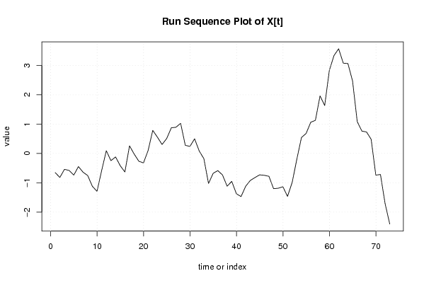
| Dataseries X: | |||||||||||||||||||||||||||||||||||||||||||||||||||||||||||||||||
-0,652 -0,818 -0,542 -0,58 -0,74 -0,448 -0,64 -0,754 -1,12 -1,292 -0,586 0,092 -0,246 -0,12 -0,42 -0,632 0,258 -0,022 -0,266 -0,324 0,1 0,786 0,554 0,304 0,508 0,874 0,892 1,026 0,276 0,238 0,498 0,082 -0,18 -1,026 -0,678 -0,586 -0,732 -1,116 -0,954 -1,376 -1,47 -1,118 -0,92 -0,822 -0,73 -0,746 -0,78 -1,202 -1,186 -1,136 -1,464 -0,99 -0,2 0,542 0,68 1,062 1,128 1,962 1,632 2,83 3,336 3,566 3,076 3,062 2,466 1,084 0,76 0,732 0,48 -0,74 -0,718 -1,712 -2,406 | |||||||||||||||||||||||||||||||||||||||||||||||||||||||||||||||||
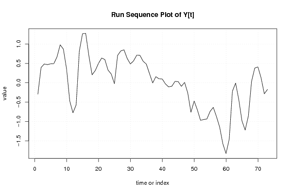
| Dataseries Y: | |||||||||||||||||||||||||||||||||||||||||||||||||||||||||||||||||
-0,294 0,394 0,486 0,47 0,49 0,494 0,67 0,982 0,87 0,356 -0,472 -0,776 -0,572 0,82 1,27 1,276 0,696 0,206 0,318 0,502 0,64 0,602 0,328 0,228 -0,024 0,708 0,824 0,852 0,632 0,486 0,566 0,714 0,71 0,558 0,484 0,238 -0,004 0,158 0,102 0,098 -0,03 -0,106 -0,09 0,036 0,03 -0,092 0,01 -0,264 -0,762 -0,472 -0,698 -0,97 -0,95 -0,936 -0,74 -0,636 -0,874 -1,146 -1,576 -1,83 -1,458 -0,218 -0,008 -0,436 -0,988 -1,222 -0,86 0,034 0,38 0,41 0,124 -0,284 -0,172 | |||||||||||||||||||||||||||||||||||||||||||||||||||||||||||||||||
Tables (Output of Computation) | |||||||||||||||||||||||||||||||||||||||||||||||||||||||||||||||||
| |||||||||||||||||||||||||||||||||||||||||||||||||||||||||||||||||
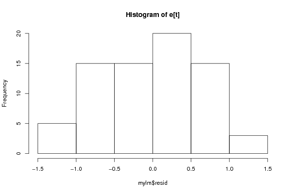
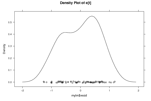
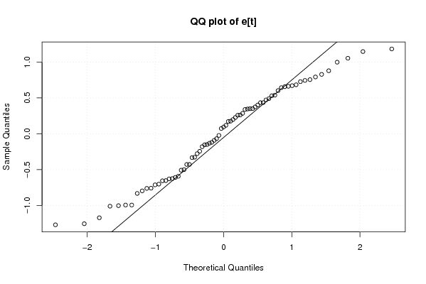
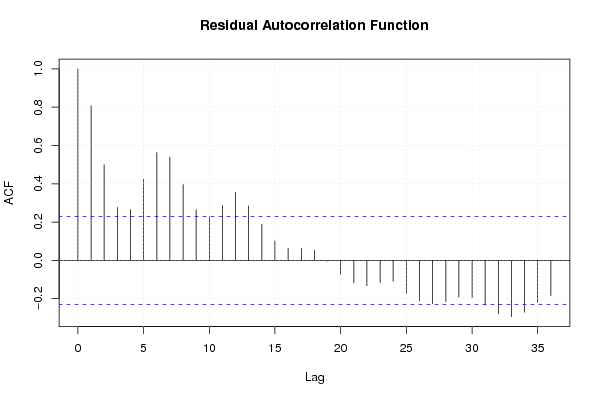
Figures (Output of Computation) | |||||||||||||||||||||||||||||||||||||||||||||||||||||||||||||||||
Input Parameters & R Code | |||||||||||||||||||||||||||||||||||||||||||||||||||||||||||||||||
| Parameters (Session): | |||||||||||||||||||||||||||||||||||||||||||||||||||||||||||||||||
| par1 = 0 ; par2 = 36 ; | |||||||||||||||||||||||||||||||||||||||||||||||||||||||||||||||||
| Parameters (R input): | |||||||||||||||||||||||||||||||||||||||||||||||||||||||||||||||||
| par1 = 0 ; par2 = 36 ; | |||||||||||||||||||||||||||||||||||||||||||||||||||||||||||||||||
| R code (references can be found in the software module): | |||||||||||||||||||||||||||||||||||||||||||||||||||||||||||||||||
par1 <- as.numeric(par1) | |||||||||||||||||||||||||||||||||||||||||||||||||||||||||||||||||