Free Statistics
of Irreproducible Research!
Description of Statistical Computation | |||||||||||||||||||||||||||||||||||||||||||||
|---|---|---|---|---|---|---|---|---|---|---|---|---|---|---|---|---|---|---|---|---|---|---|---|---|---|---|---|---|---|---|---|---|---|---|---|---|---|---|---|---|---|---|---|---|---|
| Author's title | |||||||||||||||||||||||||||||||||||||||||||||
| Author | *The author of this computation has been verified* | ||||||||||||||||||||||||||||||||||||||||||||
| R Software Module | rwasp_boxcoxlin.wasp | ||||||||||||||||||||||||||||||||||||||||||||
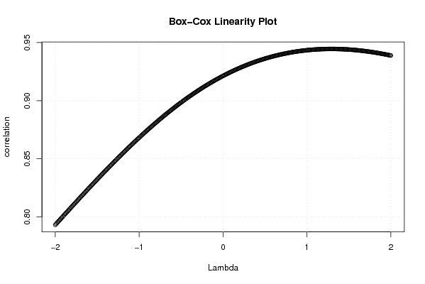
| Title produced by software | Box-Cox Linearity Plot | ||||||||||||||||||||||||||||||||||||||||||||
| Date of computation | Thu, 17 Dec 2009 22:12:56 +0100 | ||||||||||||||||||||||||||||||||||||||||||||
| Cite this page as follows | Statistical Computations at FreeStatistics.org, Office for Research Development and Education, URL https://freestatistics.org/blog/index.php?v=date/2009/Dec/17/t12610844387pu4irmjrmuvqse.htm/, Retrieved Tue, 30 Apr 2024 07:51:34 +0000 | ||||||||||||||||||||||||||||||||||||||||||||
| Statistical Computations at FreeStatistics.org, Office for Research Development and Education, URL https://freestatistics.org/blog/index.php?pk=69115, Retrieved Tue, 30 Apr 2024 07:51:34 +0000 | |||||||||||||||||||||||||||||||||||||||||||||
| QR Codes: | |||||||||||||||||||||||||||||||||||||||||||||
|
| |||||||||||||||||||||||||||||||||||||||||||||
| Original text written by user: | |||||||||||||||||||||||||||||||||||||||||||||
| IsPrivate? | No (this computation is public) | ||||||||||||||||||||||||||||||||||||||||||||
| User-defined keywords | |||||||||||||||||||||||||||||||||||||||||||||
| Estimated Impact | 157 | ||||||||||||||||||||||||||||||||||||||||||||
Tree of Dependent Computations | |||||||||||||||||||||||||||||||||||||||||||||
| Family? (F = Feedback message, R = changed R code, M = changed R Module, P = changed Parameters, D = changed Data) | |||||||||||||||||||||||||||||||||||||||||||||
| - [Univariate Data Series] [] [2009-12-17 19:09:08] [b98453cac15ba1066b407e146608df68] - RMPD [Box-Cox Linearity Plot] [] [2009-12-17 21:12:56] [d76b387543b13b5e3afd8ff9e5fdc89f] [Current] | |||||||||||||||||||||||||||||||||||||||||||||
| Feedback Forum | |||||||||||||||||||||||||||||||||||||||||||||
Post a new message | |||||||||||||||||||||||||||||||||||||||||||||
Dataset | |||||||||||||||||||||||||||||||||||||||||||||
| Dataseries X: | |||||||||||||||||||||||||||||||||||||||||||||
7.7 7.5 8.3 7.8 7.9 6.6 7 8.2 8.2 9.1 9 7.1 8.9 8.5 9.8 8.8 9.2 7.4 8.3 9.7 9.7 10.8 9.8 7.9 9.8 9 10.5 9.5 9.7 8.1 10.1 11.1 11.2 12.6 12.2 9.9 11.8 11.1 12.6 11.9 11.9 10 10.8 12.9 12.5 13.8 13.1 10.5 12.9 12.9 14.4 12.7 13.3 11 11.9 14.1 14.4 14.9 15.7 12 14.3 14.2 17.4 15.1 15.3 12.6 14 16.6 16.7 17.6 18.3 13.6 15.8 16.1 18.6 17.3 17 13.9 15.2 17.8 18 19.4 21.8 16.2 19.2 19.5 22 20 19.2 16.9 20 20.4 21.8 25 25.8 19.4 22.6 24.1 26.9 24.9 23.3 20.3 22.3 23.7 24.3 31.7 32.2 25.4 28.6 28.7 30.9 31.4 29.1 26.3 28.9 28.9 31 33.4 35.9 25.8 31.2 31.7 36.2 32 32.1 28.1 31.1 31.9 32 36.6 38.1 28.1 32.9 30.7 35.4 33.7 31.6 27.9 32.2 32.3 35.3 37.2 39.6 28.4 33.9 33.7 38.3 34.6 32.7 29.5 32 33.2 36.7 38.6 38.1 29.8 35.6 33.2 38.9 34.8 37.2 29.7 32.2 32.1 36.3 38.4 40.8 31.3 36.2 35.1 44.1 39.3 34.1 32.4 36.3 36.8 40.5 46 43.9 37.2 40.7 42 49.2 42.3 40.8 37.6 | |||||||||||||||||||||||||||||||||||||||||||||
| Dataseries Y: | |||||||||||||||||||||||||||||||||||||||||||||
277 260.6 291.6 275.4 275.3 231.7 238.8 274.2 277.8 299.1 286.6 232.3 294.1 267.5 309.7 280.7 287.3 235.7 256.4 289 290.8 321.9 291.8 241.4 295.5 258.2 306.1 281.5 283.1 237.4 274.8 299.3 300.4 340.9 318.8 265.7 322.7 281.6 323.5 312.6 310.8 262.8 273.8 320 310.3 342.2 320.1 265.6 327 300.7 346.4 317.3 326.2 270.7 278.2 324.6 321.8 343.5 354 278.2 330.2 307.3 375.9 335.3 339.3 280.3 293.7 341.2 345.1 368.7 369.4 288.4 341 319.1 374.2 344.5 337.3 281 282.2 321 325.4 366.3 380.3 300.7 359.3 327.6 383.6 352.4 329.4 294.5 333.5 334.3 358 396.1 387 307.2 363.9 344.7 397.6 376.8 337.1 299.3 323.1 329.1 347 462 436.5 360.4 415.5 382.1 432.2 424.3 386.7 354.5 375.8 368 402.4 426.5 433.3 338.5 416.8 381.1 445.7 412.4 394 348.2 380.1 373.7 393.6 434.2 430.7 344.5 411.9 370.5 437.3 411.3 385.5 341.3 384.2 373.2 415.8 448.6 454.3 350.3 419.1 398 456.1 430.1 399.8 362.7 384.9 385.3 432.3 468.9 442.7 370.2 439.4 393.9 468.7 438.8 430.1 366.3 391 380.9 431.4 465.4 471.5 387.5 446.4 421.5 504.8 492.1 421.3 396.7 428 421.9 465.6 525.8 499.9 435.3 479.5 473 554.4 489.6 462.2 420.3 | |||||||||||||||||||||||||||||||||||||||||||||
Tables (Output of Computation) | |||||||||||||||||||||||||||||||||||||||||||||
| |||||||||||||||||||||||||||||||||||||||||||||
Figures (Output of Computation) | |||||||||||||||||||||||||||||||||||||||||||||
Input Parameters & R Code | |||||||||||||||||||||||||||||||||||||||||||||
| Parameters (Session): | |||||||||||||||||||||||||||||||||||||||||||||
| par1 = FALSE ; par2 = 0.0 ; par3 = 1 ; par4 = 1 ; par5 = 12 ; par6 = 3 ; par7 = 0 ; par8 = 2 ; par9 = 1 ; | |||||||||||||||||||||||||||||||||||||||||||||
| Parameters (R input): | |||||||||||||||||||||||||||||||||||||||||||||
| R code (references can be found in the software module): | |||||||||||||||||||||||||||||||||||||||||||||
n <- length(x) | |||||||||||||||||||||||||||||||||||||||||||||