Repository of Reproducible Computations

Free Statistics

of Irreproducible Research!

Author's title

Author

*The author of this computation has been verified*

R Software Module

rwasp_autocorrelation.wasp

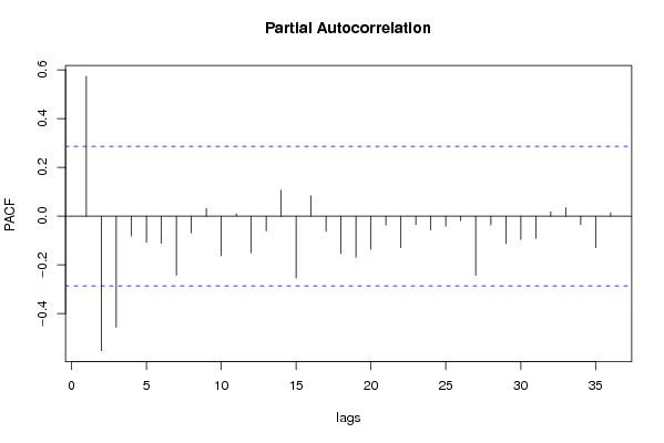
Title produced by software

(Partial) Autocorrelation Function

Date of computation

Thu, 17 Dec 2009 19:24:21 -0700

Cite this page as follows

Statistical Computations at FreeStatistics.org, Office for Research Development and Education, URL https://freestatistics.org/blog/index.php?v=date/2009/Dec/18/t1261103164vlgcpwxf6iitz2v.htm/, Retrieved Sat, 27 Apr 2024 08:33:02 +0000

Statistical Computations at FreeStatistics.org, Office for Research Development and Education, URL https://freestatistics.org/blog/index.php?pk=69150, Retrieved Sat, 27 Apr 2024 08:33:02 +0000

QR Codes:

Paste this QR Code to cite your computation.

Original text written by user:

IsPrivate?

No (this computation is public)

User-defined keywords

Estimated Impact

156

Family? (F = Feedback message, R = changed R code, M = changed R Module, P = changed Parameters, D = changed Data)

-     [Univariate Data Series] [data set] [2008-12-01 19:54:57] [b98453cac15ba1066b407e146608df68]
- RMP   [(Partial) Autocorrelation Function] [] [2009-11-27 14:47:30] [b98453cac15ba1066b407e146608df68]
-    D    [(Partial) Autocorrelation Function] [SHW WS9] [2009-12-03 16:22:00] [253127ae8da904b75450fbd69fe4eb21]
-    D      [(Partial) Autocorrelation Function] [ACF] [2009-12-04 15:00:02] [ba905ddf7cdf9ecb063c35348c4dab2e]
-    D        [(Partial) Autocorrelation Function] [] [2009-12-07 08:45:48] [ade6aa003deff66733e677339d38f25a]
-   PD            [(Partial) Autocorrelation Function] [] [2009-12-18 02:24:21] [d41d8cd98f00b204e9800998ecf8427e] [Current]

Feedback Forum

Post a new message

Dataseries X:

Download CSV

Histogram

Boxplots

9.0
9.1
8.7
8.2
7.9
7.9
9.1
9.4
9.4
9.1
9.0
9.3
9.9
9.8
9.3
8.3
8.0
8.5
10.4
11.1
10.9
10.0
9.2
9.2
9.5
9.6
9.5
9.1
8.9
9.0
10.1
10.3
10.2
9.6
9.2
9.3
9.4
9.4
9.2
9.0
9.0
9.0
9.8
10.0
9.8
9.3
9.0
9.0
9.1
9.1
9.1
9.2
8.8
8.3
8.4
8.1
7.7
7.9
7.9
8.0

Summary of computational transaction
Raw Input	view raw input (R code)
Raw Output	view raw output of R engine
Computing time	2 seconds
R Server	'Gwilym Jenkins' @ 72.249.127.135

\begin{tabular}{lllllllll}
\hline
Summary of computational transaction \tabularnewline
Raw Input & view raw input (R code)  \tabularnewline
Raw Output & view raw output of R engine  \tabularnewline
Computing time & 2 seconds \tabularnewline
R Server & 'Gwilym Jenkins' @ 72.249.127.135 \tabularnewline
\hline
\end{tabular}
%Source: https://freestatistics.org/blog/index.php?pk=69150&T=0

[TABLE]
[ROW][C]Summary of computational transaction[/C][/ROW]
[ROW][C]Raw Input[/C][C]view raw input (R code) [/C][/ROW]
[ROW][C]Raw Output[/C][C]view raw output of R engine [/C][/ROW]
[ROW][C]Computing time[/C][C]2 seconds[/C][/ROW]
[ROW][C]R Server[/C][C]'Gwilym Jenkins' @ 72.249.127.135[/C][/ROW]
[/TABLE]
Source: https://freestatistics.org/blog/index.php?pk=69150&T=0

Globally Unique Identifier (entire table): ba.freestatistics.org/blog/index.php?pk=69150&T=0

As an alternative you can also use a QR Code:

The GUIDs for individual cells are displayed in the table below:

Summary of computational transaction
Raw Input	view raw input (R code)
Raw Output	view raw output of R engine
Computing time	2 seconds
R Server	'Gwilym Jenkins' @ 72.249.127.135

Autocorrelation Function
Time lag k	ACF(k)	T-STAT	P-value
1	0.573169	3.9294	0.000139
2	-0.042103	-0.2886	0.387062
3	-0.566512	-3.8838	0.00016
4	-0.646782	-4.4341	2.8e-05
5	-0.368078	-2.5234	0.007531
6	0.049312	0.3381	0.368409
7	0.279244	1.9144	0.030834
8	0.306761	2.1031	0.020421
9	0.19366	1.3277	0.09535
10	0.002143	0.0147	0.49417
11	-0.0998	-0.6842	0.248607
12	-0.169861	-1.1645	0.125048
13	-0.143666	-0.9849	0.164852
14	-0.018028	-0.1236	0.451083
15	0.037776	0.259	0.398391
16	0.102873	0.7053	0.242064
17	0.084467	0.5791	0.282651
18	0.006809	0.0467	0.481484
19	-0.113924	-0.781	0.219352
20	-0.12887	-0.8835	0.190734
21	-0.071778	-0.4921	0.312475
22	0.067902	0.4655	0.321857
23	0.190386	1.3052	0.099086
24	0.176762	1.2118	0.115819
25	0.082451	0.5653	0.287295
26	-0.080746	-0.5536	0.291251
27	-0.221319	-1.5173	0.067946
28	-0.212355	-1.4558	0.076044
29	-0.098757	-0.677	0.250849
30	0.086609	0.5938	0.27776
31	0.216453	1.4839	0.072252
32	0.267203	1.8319	0.036657
33	0.147657	1.0123	0.158292
34	-0.010451	-0.0717	0.471592
35	-0.220181	-1.5095	0.068934
36	-0.283866	-1.9461	0.028818

\begin{tabular}{lllllllll}
\hline
Autocorrelation Function \tabularnewline
Time lag k & ACF(k) & T-STAT & P-value \tabularnewline
1 & 0.573169 & 3.9294 & 0.000139 \tabularnewline
2 & -0.042103 & -0.2886 & 0.387062 \tabularnewline
3 & -0.566512 & -3.8838 & 0.00016 \tabularnewline
4 & -0.646782 & -4.4341 & 2.8e-05 \tabularnewline
5 & -0.368078 & -2.5234 & 0.007531 \tabularnewline
6 & 0.049312 & 0.3381 & 0.368409 \tabularnewline
7 & 0.279244 & 1.9144 & 0.030834 \tabularnewline
8 & 0.306761 & 2.1031 & 0.020421 \tabularnewline
9 & 0.19366 & 1.3277 & 0.09535 \tabularnewline
10 & 0.002143 & 0.0147 & 0.49417 \tabularnewline
11 & -0.0998 & -0.6842 & 0.248607 \tabularnewline
12 & -0.169861 & -1.1645 & 0.125048 \tabularnewline
13 & -0.143666 & -0.9849 & 0.164852 \tabularnewline
14 & -0.018028 & -0.1236 & 0.451083 \tabularnewline
15 & 0.037776 & 0.259 & 0.398391 \tabularnewline
16 & 0.102873 & 0.7053 & 0.242064 \tabularnewline
17 & 0.084467 & 0.5791 & 0.282651 \tabularnewline
18 & 0.006809 & 0.0467 & 0.481484 \tabularnewline
19 & -0.113924 & -0.781 & 0.219352 \tabularnewline
20 & -0.12887 & -0.8835 & 0.190734 \tabularnewline
21 & -0.071778 & -0.4921 & 0.312475 \tabularnewline
22 & 0.067902 & 0.4655 & 0.321857 \tabularnewline
23 & 0.190386 & 1.3052 & 0.099086 \tabularnewline
24 & 0.176762 & 1.2118 & 0.115819 \tabularnewline
25 & 0.082451 & 0.5653 & 0.287295 \tabularnewline
26 & -0.080746 & -0.5536 & 0.291251 \tabularnewline
27 & -0.221319 & -1.5173 & 0.067946 \tabularnewline
28 & -0.212355 & -1.4558 & 0.076044 \tabularnewline
29 & -0.098757 & -0.677 & 0.250849 \tabularnewline
30 & 0.086609 & 0.5938 & 0.27776 \tabularnewline
31 & 0.216453 & 1.4839 & 0.072252 \tabularnewline
32 & 0.267203 & 1.8319 & 0.036657 \tabularnewline
33 & 0.147657 & 1.0123 & 0.158292 \tabularnewline
34 & -0.010451 & -0.0717 & 0.471592 \tabularnewline
35 & -0.220181 & -1.5095 & 0.068934 \tabularnewline
36 & -0.283866 & -1.9461 & 0.028818 \tabularnewline
\hline
\end{tabular}
%Source: https://freestatistics.org/blog/index.php?pk=69150&T=1

[TABLE]
[ROW][C]Autocorrelation Function[/C][/ROW]
[ROW][C]Time lag k[/C][C]ACF(k)[/C][C]T-STAT[/C][C]P-value[/C][/ROW]
[ROW][C]1[/C][C]0.573169[/C][C]3.9294[/C][C]0.000139[/C][/ROW]
[ROW][C]2[/C][C]-0.042103[/C][C]-0.2886[/C][C]0.387062[/C][/ROW]
[ROW][C]3[/C][C]-0.566512[/C][C]-3.8838[/C][C]0.00016[/C][/ROW]
[ROW][C]4[/C][C]-0.646782[/C][C]-4.4341[/C][C]2.8e-05[/C][/ROW]
[ROW][C]5[/C][C]-0.368078[/C][C]-2.5234[/C][C]0.007531[/C][/ROW]
[ROW][C]6[/C][C]0.049312[/C][C]0.3381[/C][C]0.368409[/C][/ROW]
[ROW][C]7[/C][C]0.279244[/C][C]1.9144[/C][C]0.030834[/C][/ROW]
[ROW][C]8[/C][C]0.306761[/C][C]2.1031[/C][C]0.020421[/C][/ROW]
[ROW][C]9[/C][C]0.19366[/C][C]1.3277[/C][C]0.09535[/C][/ROW]
[ROW][C]10[/C][C]0.002143[/C][C]0.0147[/C][C]0.49417[/C][/ROW]
[ROW][C]11[/C][C]-0.0998[/C][C]-0.6842[/C][C]0.248607[/C][/ROW]
[ROW][C]12[/C][C]-0.169861[/C][C]-1.1645[/C][C]0.125048[/C][/ROW]
[ROW][C]13[/C][C]-0.143666[/C][C]-0.9849[/C][C]0.164852[/C][/ROW]
[ROW][C]14[/C][C]-0.018028[/C][C]-0.1236[/C][C]0.451083[/C][/ROW]
[ROW][C]15[/C][C]0.037776[/C][C]0.259[/C][C]0.398391[/C][/ROW]
[ROW][C]16[/C][C]0.102873[/C][C]0.7053[/C][C]0.242064[/C][/ROW]
[ROW][C]17[/C][C]0.084467[/C][C]0.5791[/C][C]0.282651[/C][/ROW]
[ROW][C]18[/C][C]0.006809[/C][C]0.0467[/C][C]0.481484[/C][/ROW]
[ROW][C]19[/C][C]-0.113924[/C][C]-0.781[/C][C]0.219352[/C][/ROW]
[ROW][C]20[/C][C]-0.12887[/C][C]-0.8835[/C][C]0.190734[/C][/ROW]
[ROW][C]21[/C][C]-0.071778[/C][C]-0.4921[/C][C]0.312475[/C][/ROW]
[ROW][C]22[/C][C]0.067902[/C][C]0.4655[/C][C]0.321857[/C][/ROW]
[ROW][C]23[/C][C]0.190386[/C][C]1.3052[/C][C]0.099086[/C][/ROW]
[ROW][C]24[/C][C]0.176762[/C][C]1.2118[/C][C]0.115819[/C][/ROW]
[ROW][C]25[/C][C]0.082451[/C][C]0.5653[/C][C]0.287295[/C][/ROW]
[ROW][C]26[/C][C]-0.080746[/C][C]-0.5536[/C][C]0.291251[/C][/ROW]
[ROW][C]27[/C][C]-0.221319[/C][C]-1.5173[/C][C]0.067946[/C][/ROW]
[ROW][C]28[/C][C]-0.212355[/C][C]-1.4558[/C][C]0.076044[/C][/ROW]
[ROW][C]29[/C][C]-0.098757[/C][C]-0.677[/C][C]0.250849[/C][/ROW]
[ROW][C]30[/C][C]0.086609[/C][C]0.5938[/C][C]0.27776[/C][/ROW]
[ROW][C]31[/C][C]0.216453[/C][C]1.4839[/C][C]0.072252[/C][/ROW]
[ROW][C]32[/C][C]0.267203[/C][C]1.8319[/C][C]0.036657[/C][/ROW]
[ROW][C]33[/C][C]0.147657[/C][C]1.0123[/C][C]0.158292[/C][/ROW]
[ROW][C]34[/C][C]-0.010451[/C][C]-0.0717[/C][C]0.471592[/C][/ROW]
[ROW][C]35[/C][C]-0.220181[/C][C]-1.5095[/C][C]0.068934[/C][/ROW]
[ROW][C]36[/C][C]-0.283866[/C][C]-1.9461[/C][C]0.028818[/C][/ROW]
[/TABLE]
Source: https://freestatistics.org/blog/index.php?pk=69150&T=1

Globally Unique Identifier (entire table): ba.freestatistics.org/blog/index.php?pk=69150&T=1

As an alternative you can also use a QR Code:

The GUIDs for individual cells are displayed in the table below:

Autocorrelation Function
Time lag k	ACF(k)	T-STAT	P-value
1	0.573169	3.9294	0.000139
2	-0.042103	-0.2886	0.387062
3	-0.566512	-3.8838	0.00016
4	-0.646782	-4.4341	2.8e-05
5	-0.368078	-2.5234	0.007531
6	0.049312	0.3381	0.368409
7	0.279244	1.9144	0.030834
8	0.306761	2.1031	0.020421
9	0.19366	1.3277	0.09535
10	0.002143	0.0147	0.49417
11	-0.0998	-0.6842	0.248607
12	-0.169861	-1.1645	0.125048
13	-0.143666	-0.9849	0.164852
14	-0.018028	-0.1236	0.451083
15	0.037776	0.259	0.398391
16	0.102873	0.7053	0.242064
17	0.084467	0.5791	0.282651
18	0.006809	0.0467	0.481484
19	-0.113924	-0.781	0.219352
20	-0.12887	-0.8835	0.190734
21	-0.071778	-0.4921	0.312475
22	0.067902	0.4655	0.321857
23	0.190386	1.3052	0.099086
24	0.176762	1.2118	0.115819
25	0.082451	0.5653	0.287295
26	-0.080746	-0.5536	0.291251
27	-0.221319	-1.5173	0.067946
28	-0.212355	-1.4558	0.076044
29	-0.098757	-0.677	0.250849
30	0.086609	0.5938	0.27776
31	0.216453	1.4839	0.072252
32	0.267203	1.8319	0.036657
33	0.147657	1.0123	0.158292
34	-0.010451	-0.0717	0.471592
35	-0.220181	-1.5095	0.068934
36	-0.283866	-1.9461	0.028818

Partial Autocorrelation Function
Time lag k	PACF(k)	T-STAT	P-value
1	0.573169	3.9294	0.000139
2	-0.551956	-3.784	0.000218
3	-0.455542	-3.123	0.001531
4	-0.082076	-0.5627	0.288161
5	-0.107297	-0.7356	0.232817
6	-0.112286	-0.7698	0.222636
7	-0.242363	-1.6616	0.05163
8	-0.068179	-0.4674	0.321182
9	0.031578	0.2165	0.414772
10	-0.162343	-1.113	0.135691
11	0.009469	0.0649	0.474259
12	-0.150088	-1.029	0.154384
13	-0.06031	-0.4135	0.340574
14	0.106576	0.7306	0.234311
15	-0.253955	-1.741	0.044111
16	0.083521	0.5726	0.284826
17	-0.062925	-0.4314	0.334079
18	-0.153597	-1.053	0.148861
19	-0.169144	-1.1596	0.126037
20	-0.135157	-0.9266	0.179436
21	-0.037262	-0.2555	0.399744
22	-0.129859	-0.8903	0.188929
23	-0.035452	-0.243	0.404514
24	-0.056703	-0.3887	0.349614
25	-0.04099	-0.281	0.389966
26	-0.019216	-0.1317	0.447877
27	-0.242961	-1.6657	0.051217
28	-0.035776	-0.2453	0.403659
29	-0.113423	-0.7776	0.220355
30	-0.09605	-0.6585	0.256719
31	-0.091144	-0.6249	0.267545
32	0.017783	0.1219	0.451742
33	0.03434	0.2354	0.407451
34	-0.035597	-0.244	0.404131
35	-0.129906	-0.8906	0.188843
36	0.014023	0.0961	0.461912

\begin{tabular}{lllllllll}
\hline
Partial Autocorrelation Function \tabularnewline
Time lag k & PACF(k) & T-STAT & P-value \tabularnewline
1 & 0.573169 & 3.9294 & 0.000139 \tabularnewline
2 & -0.551956 & -3.784 & 0.000218 \tabularnewline
3 & -0.455542 & -3.123 & 0.001531 \tabularnewline
4 & -0.082076 & -0.5627 & 0.288161 \tabularnewline
5 & -0.107297 & -0.7356 & 0.232817 \tabularnewline
6 & -0.112286 & -0.7698 & 0.222636 \tabularnewline
7 & -0.242363 & -1.6616 & 0.05163 \tabularnewline
8 & -0.068179 & -0.4674 & 0.321182 \tabularnewline
9 & 0.031578 & 0.2165 & 0.414772 \tabularnewline
10 & -0.162343 & -1.113 & 0.135691 \tabularnewline
11 & 0.009469 & 0.0649 & 0.474259 \tabularnewline
12 & -0.150088 & -1.029 & 0.154384 \tabularnewline
13 & -0.06031 & -0.4135 & 0.340574 \tabularnewline
14 & 0.106576 & 0.7306 & 0.234311 \tabularnewline
15 & -0.253955 & -1.741 & 0.044111 \tabularnewline
16 & 0.083521 & 0.5726 & 0.284826 \tabularnewline
17 & -0.062925 & -0.4314 & 0.334079 \tabularnewline
18 & -0.153597 & -1.053 & 0.148861 \tabularnewline
19 & -0.169144 & -1.1596 & 0.126037 \tabularnewline
20 & -0.135157 & -0.9266 & 0.179436 \tabularnewline
21 & -0.037262 & -0.2555 & 0.399744 \tabularnewline
22 & -0.129859 & -0.8903 & 0.188929 \tabularnewline
23 & -0.035452 & -0.243 & 0.404514 \tabularnewline
24 & -0.056703 & -0.3887 & 0.349614 \tabularnewline
25 & -0.04099 & -0.281 & 0.389966 \tabularnewline
26 & -0.019216 & -0.1317 & 0.447877 \tabularnewline
27 & -0.242961 & -1.6657 & 0.051217 \tabularnewline
28 & -0.035776 & -0.2453 & 0.403659 \tabularnewline
29 & -0.113423 & -0.7776 & 0.220355 \tabularnewline
30 & -0.09605 & -0.6585 & 0.256719 \tabularnewline
31 & -0.091144 & -0.6249 & 0.267545 \tabularnewline
32 & 0.017783 & 0.1219 & 0.451742 \tabularnewline
33 & 0.03434 & 0.2354 & 0.407451 \tabularnewline
34 & -0.035597 & -0.244 & 0.404131 \tabularnewline
35 & -0.129906 & -0.8906 & 0.188843 \tabularnewline
36 & 0.014023 & 0.0961 & 0.461912 \tabularnewline
\hline
\end{tabular}
%Source: https://freestatistics.org/blog/index.php?pk=69150&T=2

[TABLE]
[ROW][C]Partial Autocorrelation Function[/C][/ROW]
[ROW][C]Time lag k[/C][C]PACF(k)[/C][C]T-STAT[/C][C]P-value[/C][/ROW]
[ROW][C]1[/C][C]0.573169[/C][C]3.9294[/C][C]0.000139[/C][/ROW]
[ROW][C]2[/C][C]-0.551956[/C][C]-3.784[/C][C]0.000218[/C][/ROW]
[ROW][C]3[/C][C]-0.455542[/C][C]-3.123[/C][C]0.001531[/C][/ROW]
[ROW][C]4[/C][C]-0.082076[/C][C]-0.5627[/C][C]0.288161[/C][/ROW]
[ROW][C]5[/C][C]-0.107297[/C][C]-0.7356[/C][C]0.232817[/C][/ROW]
[ROW][C]6[/C][C]-0.112286[/C][C]-0.7698[/C][C]0.222636[/C][/ROW]
[ROW][C]7[/C][C]-0.242363[/C][C]-1.6616[/C][C]0.05163[/C][/ROW]
[ROW][C]8[/C][C]-0.068179[/C][C]-0.4674[/C][C]0.321182[/C][/ROW]
[ROW][C]9[/C][C]0.031578[/C][C]0.2165[/C][C]0.414772[/C][/ROW]
[ROW][C]10[/C][C]-0.162343[/C][C]-1.113[/C][C]0.135691[/C][/ROW]
[ROW][C]11[/C][C]0.009469[/C][C]0.0649[/C][C]0.474259[/C][/ROW]
[ROW][C]12[/C][C]-0.150088[/C][C]-1.029[/C][C]0.154384[/C][/ROW]
[ROW][C]13[/C][C]-0.06031[/C][C]-0.4135[/C][C]0.340574[/C][/ROW]
[ROW][C]14[/C][C]0.106576[/C][C]0.7306[/C][C]0.234311[/C][/ROW]
[ROW][C]15[/C][C]-0.253955[/C][C]-1.741[/C][C]0.044111[/C][/ROW]
[ROW][C]16[/C][C]0.083521[/C][C]0.5726[/C][C]0.284826[/C][/ROW]
[ROW][C]17[/C][C]-0.062925[/C][C]-0.4314[/C][C]0.334079[/C][/ROW]
[ROW][C]18[/C][C]-0.153597[/C][C]-1.053[/C][C]0.148861[/C][/ROW]
[ROW][C]19[/C][C]-0.169144[/C][C]-1.1596[/C][C]0.126037[/C][/ROW]
[ROW][C]20[/C][C]-0.135157[/C][C]-0.9266[/C][C]0.179436[/C][/ROW]
[ROW][C]21[/C][C]-0.037262[/C][C]-0.2555[/C][C]0.399744[/C][/ROW]
[ROW][C]22[/C][C]-0.129859[/C][C]-0.8903[/C][C]0.188929[/C][/ROW]
[ROW][C]23[/C][C]-0.035452[/C][C]-0.243[/C][C]0.404514[/C][/ROW]
[ROW][C]24[/C][C]-0.056703[/C][C]-0.3887[/C][C]0.349614[/C][/ROW]
[ROW][C]25[/C][C]-0.04099[/C][C]-0.281[/C][C]0.389966[/C][/ROW]
[ROW][C]26[/C][C]-0.019216[/C][C]-0.1317[/C][C]0.447877[/C][/ROW]
[ROW][C]27[/C][C]-0.242961[/C][C]-1.6657[/C][C]0.051217[/C][/ROW]
[ROW][C]28[/C][C]-0.035776[/C][C]-0.2453[/C][C]0.403659[/C][/ROW]
[ROW][C]29[/C][C]-0.113423[/C][C]-0.7776[/C][C]0.220355[/C][/ROW]
[ROW][C]30[/C][C]-0.09605[/C][C]-0.6585[/C][C]0.256719[/C][/ROW]
[ROW][C]31[/C][C]-0.091144[/C][C]-0.6249[/C][C]0.267545[/C][/ROW]
[ROW][C]32[/C][C]0.017783[/C][C]0.1219[/C][C]0.451742[/C][/ROW]
[ROW][C]33[/C][C]0.03434[/C][C]0.2354[/C][C]0.407451[/C][/ROW]
[ROW][C]34[/C][C]-0.035597[/C][C]-0.244[/C][C]0.404131[/C][/ROW]
[ROW][C]35[/C][C]-0.129906[/C][C]-0.8906[/C][C]0.188843[/C][/ROW]
[ROW][C]36[/C][C]0.014023[/C][C]0.0961[/C][C]0.461912[/C][/ROW]
[/TABLE]
Source: https://freestatistics.org/blog/index.php?pk=69150&T=2

Globally Unique Identifier (entire table): ba.freestatistics.org/blog/index.php?pk=69150&T=2

As an alternative you can also use a QR Code:

The GUIDs for individual cells are displayed in the table below:

Partial Autocorrelation Function
Time lag k	PACF(k)	T-STAT	P-value
1	0.573169	3.9294	0.000139
2	-0.551956	-3.784	0.000218
3	-0.455542	-3.123	0.001531
4	-0.082076	-0.5627	0.288161
5	-0.107297	-0.7356	0.232817
6	-0.112286	-0.7698	0.222636
7	-0.242363	-1.6616	0.05163
8	-0.068179	-0.4674	0.321182
9	0.031578	0.2165	0.414772
10	-0.162343	-1.113	0.135691
11	0.009469	0.0649	0.474259
12	-0.150088	-1.029	0.154384
13	-0.06031	-0.4135	0.340574
14	0.106576	0.7306	0.234311
15	-0.253955	-1.741	0.044111
16	0.083521	0.5726	0.284826
17	-0.062925	-0.4314	0.334079
18	-0.153597	-1.053	0.148861
19	-0.169144	-1.1596	0.126037
20	-0.135157	-0.9266	0.179436
21	-0.037262	-0.2555	0.399744
22	-0.129859	-0.8903	0.188929
23	-0.035452	-0.243	0.404514
24	-0.056703	-0.3887	0.349614
25	-0.04099	-0.281	0.389966
26	-0.019216	-0.1317	0.447877
27	-0.242961	-1.6657	0.051217
28	-0.035776	-0.2453	0.403659
29	-0.113423	-0.7776	0.220355
30	-0.09605	-0.6585	0.256719
31	-0.091144	-0.6249	0.267545
32	0.017783	0.1219	0.451742
33	0.03434	0.2354	0.407451
34	-0.035597	-0.244	0.404131
35	-0.129906	-0.8906	0.188843
36	0.014023	0.0961	0.461912

Figure 1

PNG link

Postscript link

PDF link

Figure 2

PNG link

Postscript link

PDF link

Parameters (Session):

par1 = 36 ; par2 = 1 ; par3 = 1 ; par4 = 1 ; par5 = 12 ; par6 = MA ; par7 = 0.95 ;

Parameters (R input):

par1 = 36 ; par2 = 1 ; par3 = 1 ; par4 = 1 ; par5 = 12 ; par6 = MA ; par7 = 0.95 ;

R code (references can be found in the software module):

if (par1 == 'Default') {
par1 = 10*log10(length(x))
} else {
par1 <- as.numeric(par1)
}
par2 <- as.numeric(par2)
par3 <- as.numeric(par3)
par4 <- as.numeric(par4)
par5 <- as.numeric(par5)
if (par6 == 'White Noise') par6 <- 'white' else par6 <- 'ma'
par7 <- as.numeric(par7)
if (par2 == 0) {
x <- log(x)
} else {
x <- (x ^ par2 - 1) / par2
}
if (par3 > 0) x <- diff(x,lag=1,difference=par3)
if (par4 > 0) x <- diff(x,lag=par5,difference=par4)
bitmap(file='pic1.png')
racf <- acf(x, par1, main='Autocorrelation', xlab='time lag', ylab='ACF', ci.type=par6, ci=par7, sub=paste('(lambda=',par2,', d=',par3,', D=',par4,', CI=', par7, ', CI type=',par6,')',sep=''))
dev.off()
bitmap(file='pic2.png')
rpacf <- pacf(x,par1,main='Partial Autocorrelation',xlab='lags',ylab='PACF')
dev.off()
(myacf <- c(racf$acf))
(mypacf <- c(rpacf$acf))
lengthx <- length(x)
sqrtn <- sqrt(lengthx)
load(file='createtable')
a<-table.start()
a<-table.row.start(a)
a<-table.element(a,'Autocorrelation Function',4,TRUE)
a<-table.row.end(a)
a<-table.row.start(a)
a<-table.element(a,'Time lag k',header=TRUE)
a<-table.element(a,hyperlink('basics.htm','ACF(k)','click here for more information about the Autocorrelation Function'),header=TRUE)
a<-table.element(a,'T-STAT',header=TRUE)
a<-table.element(a,'P-value',header=TRUE)
a<-table.row.end(a)
for (i in 2:(par1+1)) {
a<-table.row.start(a)
a<-table.element(a,i-1,header=TRUE)
a<-table.element(a,round(myacf[i],6))
mytstat <- myacf[i]*sqrtn
a<-table.element(a,round(mytstat,4))
a<-table.element(a,round(1-pt(abs(mytstat),lengthx),6))
a<-table.row.end(a)
}
a<-table.end(a)
table.save(a,file='mytable.tab')
a<-table.start()
a<-table.row.start(a)
a<-table.element(a,'Partial Autocorrelation Function',4,TRUE)
a<-table.row.end(a)
a<-table.row.start(a)
a<-table.element(a,'Time lag k',header=TRUE)
a<-table.element(a,hyperlink('basics.htm','PACF(k)','click here for more information about the Partial Autocorrelation Function'),header=TRUE)
a<-table.element(a,'T-STAT',header=TRUE)
a<-table.element(a,'P-value',header=TRUE)
a<-table.row.end(a)
for (i in 1:par1) {
a<-table.row.start(a)
a<-table.element(a,i,header=TRUE)
a<-table.element(a,round(mypacf[i],6))
mytstat <- mypacf[i]*sqrtn
a<-table.element(a,round(mytstat,4))
a<-table.element(a,round(1-pt(abs(mytstat),lengthx),6))
a<-table.row.end(a)
}
a<-table.end(a)
table.save(a,file='mytable1.tab')

Free Statistics

Description of Statistical Computation

Tree of Dependent Computations

Dataset

Tables (Output of Computation)

Figures (Output of Computation)

Input Parameters & R Code