Repository of Reproducible Computations

Free Statistics

of Irreproducible Research!

Author's title

Author

*The author of this computation has been verified*

R Software Module

rwasp_edauni.wasp

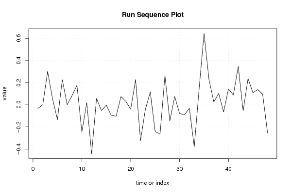
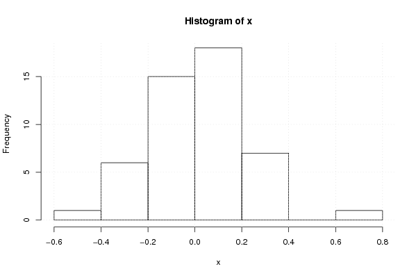
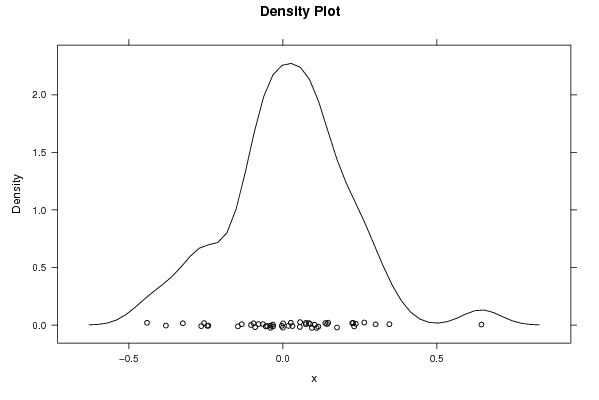
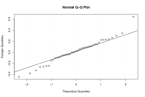
Title produced by software

Univariate Explorative Data Analysis

Date of computation

Fri, 18 Dec 2009 03:48:30 -0700

Cite this page as follows

Statistical Computations at FreeStatistics.org, Office for Research Development and Education, URL https://freestatistics.org/blog/index.php?v=date/2009/Dec/18/t1261133414t40lzka1i2mij6i.htm/, Retrieved Sat, 27 Apr 2024 05:48:07 +0000

Statistical Computations at FreeStatistics.org, Office for Research Development and Education, URL https://freestatistics.org/blog/index.php?pk=69218, Retrieved Sat, 27 Apr 2024 05:48:07 +0000

QR Codes:

Paste this QR Code to cite your computation.

Original text written by user:

IsPrivate?

No (this computation is public)

User-defined keywords

Estimated Impact

138

Family? (F = Feedback message, R = changed R code, M = changed R Module, P = changed Parameters, D = changed Data)

-     [Bivariate Data Series] [Bivariate dataset] [2008-01-05 23:51:08] [74be16979710d4c4e7c6647856088456]
- RMPD  [Univariate Explorative Data Analysis] [SHW_WS4_Q3] [2009-10-23 09:32:44] [8b1aef4e7013bd33fbc2a5833375c5f5]
-  M D    [Univariate Explorative Data Analysis] [paper] [2009-11-29 11:29:44] [b5908418e3090fddbd22f5f0f774653d]
-    D        [Univariate Explorative Data Analysis] [paper] [2009-12-18 10:48:30] [f7d3e79b917995ba1c8c80042fc22ef9] [Current]

Feedback Forum

Post a new message

Dataseries X:

Download CSV

Histogram

Boxplots

-0.0322477563269516
-3.10259255310256e-05
0.301112186970538
0.0548018747461919
-0.133474622792253
0.225291776937562
0.000852895716111257
0.084341638102194
0.175638628134376
-0.245187524575567
0.0183476060840533
-0.440793105929656
0.05602794751164
-0.0510397796031188
-0.00363943386617446
-0.0951080672001434
-0.103351045622180
0.0742974455944183
0.0310716492059746
-0.039678164485403
0.227962566341790
-0.324561783178065
-0.039986746601846
0.115065195584166
-0.241826610194115
-0.265010543596649
0.264312619508534
-0.145748811773052
0.074984846215623
-0.0792037460618129
-0.0897138675350125
-0.0318891439749827
-0.379520044986777
0.147081259023469
0.644573158872214
0.231406353542911
0.0257968317972824
0.102825006570345
-0.0644471569186438
0.143283137022815
0.088575110656249
0.345773687682914
-0.0556153301369342
0.236619255674046
0.109662493707481
0.137836003726974
0.0941980971503112
-0.255678058936345

Summary of computational transaction
Raw Input	view raw input (R code)
Raw Output	view raw output of R engine
Computing time	3 seconds
R Server	'Gwilym Jenkins' @ 72.249.127.135

\begin{tabular}{lllllllll}
\hline
Summary of computational transaction \tabularnewline
Raw Input & view raw input (R code)  \tabularnewline
Raw Output & view raw output of R engine  \tabularnewline
Computing time & 3 seconds \tabularnewline
R Server & 'Gwilym Jenkins' @ 72.249.127.135 \tabularnewline
\hline
\end{tabular}
%Source: https://freestatistics.org/blog/index.php?pk=69218&T=0

[TABLE]
[ROW][C]Summary of computational transaction[/C][/ROW]
[ROW][C]Raw Input[/C][C]view raw input (R code) [/C][/ROW]
[ROW][C]Raw Output[/C][C]view raw output of R engine [/C][/ROW]
[ROW][C]Computing time[/C][C]3 seconds[/C][/ROW]
[ROW][C]R Server[/C][C]'Gwilym Jenkins' @ 72.249.127.135[/C][/ROW]
[/TABLE]
Source: https://freestatistics.org/blog/index.php?pk=69218&T=0

Globally Unique Identifier (entire table): ba.freestatistics.org/blog/index.php?pk=69218&T=0

As an alternative you can also use a QR Code:

The GUIDs for individual cells are displayed in the table below:

Summary of computational transaction
Raw Input	view raw input (R code)
Raw Output	view raw output of R engine
Computing time	3 seconds
R Server	'Gwilym Jenkins' @ 72.249.127.135

Descriptive Statistics
# observations	48
minimum	-0.440793105929656
Q1	-0.0818312764301128
median	0.0220722189406679
mean	0.0186247271220619
Q3	0.120757897619868
maximum	0.644573158872214

\begin{tabular}{lllllllll}
\hline
Descriptive Statistics \tabularnewline
# observations & 48 \tabularnewline
minimum & -0.440793105929656 \tabularnewline
Q1 & -0.0818312764301128 \tabularnewline
median & 0.0220722189406679 \tabularnewline
mean & 0.0186247271220619 \tabularnewline
Q3 & 0.120757897619868 \tabularnewline
maximum & 0.644573158872214 \tabularnewline
\hline
\end{tabular}
%Source: https://freestatistics.org/blog/index.php?pk=69218&T=1

[TABLE]
[ROW][C]Descriptive Statistics[/C][/ROW]
[ROW][C]# observations[/C][C]48[/C][/ROW]
[ROW][C]minimum[/C][C]-0.440793105929656[/C][/ROW]
[ROW][C]Q1[/C][C]-0.0818312764301128[/C][/ROW]
[ROW][C]median[/C][C]0.0220722189406679[/C][/ROW]
[ROW][C]mean[/C][C]0.0186247271220619[/C][/ROW]
[ROW][C]Q3[/C][C]0.120757897619868[/C][/ROW]
[ROW][C]maximum[/C][C]0.644573158872214[/C][/ROW]
[/TABLE]
Source: https://freestatistics.org/blog/index.php?pk=69218&T=1

Globally Unique Identifier (entire table): ba.freestatistics.org/blog/index.php?pk=69218&T=1

As an alternative you can also use a QR Code:

The GUIDs for individual cells are displayed in the table below:

Descriptive Statistics
# observations	48
minimum	-0.440793105929656
Q1	-0.0818312764301128
median	0.0220722189406679
mean	0.0186247271220619
Q3	0.120757897619868
maximum	0.644573158872214

Figure 1

PNG link

Postscript link

PDF link

Figure 2

PNG link

Postscript link

PDF link

Figure 3

PNG link

Postscript link

PDF link

Figure 4

PNG link

Postscript link

PDF link

Figure 5

PNG link

Postscript link

PDF link

Figure 6

PNG link

Postscript link

PDF link

Figure 7

PNG link

Postscript link

PDF link

Parameters (Session):

par1 = 0 ; par2 = 36 ;

Parameters (R input):

par1 = 0 ; par2 = 36 ;

R code (references can be found in the software module):

par1 <- as.numeric(par1)
par2 <- as.numeric(par2)
x <- as.ts(x)
library(lattice)
bitmap(file='pic1.png')
plot(x,type='l',main='Run Sequence Plot',xlab='time or index',ylab='value')
grid()
dev.off()
bitmap(file='pic2.png')
hist(x)
grid()
dev.off()
bitmap(file='pic3.png')
if (par1 > 0)
{
densityplot(~x,col='black',main=paste('Density Plot   bw = ',par1),bw=par1)
} else {
densityplot(~x,col='black',main='Density Plot')
}
dev.off()
bitmap(file='pic4.png')
qqnorm(x)
qqline(x)
grid()
dev.off()
if (par2 > 0)
{
bitmap(file='lagplot1.png')
dum <- cbind(lag(x,k=1),x)
dum
dum1 <- dum[2:length(x),]
dum1
z <- as.data.frame(dum1)
z
plot(z,main='Lag plot (k=1), lowess, and regression line')
lines(lowess(z))
abline(lm(z))
dev.off()
if (par2 > 1) {
bitmap(file='lagplotpar2.png')
dum <- cbind(lag(x,k=par2),x)
dum
dum1 <- dum[(par2+1):length(x),]
dum1
z <- as.data.frame(dum1)
z
mylagtitle <- 'Lag plot (k='
mylagtitle <- paste(mylagtitle,par2,sep='')
mylagtitle <- paste(mylagtitle,'), and lowess',sep='')
plot(z,main=mylagtitle)
lines(lowess(z))
dev.off()
}
bitmap(file='pic5.png')
acf(x,lag.max=par2,main='Autocorrelation Function')
grid()
dev.off()
}
summary(x)
load(file='createtable')
a<-table.start()
a<-table.row.start(a)
a<-table.element(a,'Descriptive Statistics',2,TRUE)
a<-table.row.end(a)
a<-table.row.start(a)
a<-table.element(a,'# observations',header=TRUE)
a<-table.element(a,length(x))
a<-table.row.end(a)
a<-table.row.start(a)
a<-table.element(a,'minimum',header=TRUE)
a<-table.element(a,min(x))
a<-table.row.end(a)
a<-table.row.start(a)
a<-table.element(a,'Q1',header=TRUE)
a<-table.element(a,quantile(x,0.25))
a<-table.row.end(a)
a<-table.row.start(a)
a<-table.element(a,'median',header=TRUE)
a<-table.element(a,median(x))
a<-table.row.end(a)
a<-table.row.start(a)
a<-table.element(a,'mean',header=TRUE)
a<-table.element(a,mean(x))
a<-table.row.end(a)
a<-table.row.start(a)
a<-table.element(a,'Q3',header=TRUE)
a<-table.element(a,quantile(x,0.75))
a<-table.row.end(a)
a<-table.row.start(a)
a<-table.element(a,'maximum',header=TRUE)
a<-table.element(a,max(x))
a<-table.row.end(a)
a<-table.end(a)
table.save(a,file='mytable.tab')

Free Statistics

Description of Statistical Computation

Tree of Dependent Computations

Dataset

Tables (Output of Computation)

Figures (Output of Computation)

Input Parameters & R Code