Free Statistics
of Irreproducible Research!
Description of Statistical Computation | |||||||||||||||||||||||||||||||||||||||||||||||||||||
|---|---|---|---|---|---|---|---|---|---|---|---|---|---|---|---|---|---|---|---|---|---|---|---|---|---|---|---|---|---|---|---|---|---|---|---|---|---|---|---|---|---|---|---|---|---|---|---|---|---|---|---|---|---|
| Author's title | |||||||||||||||||||||||||||||||||||||||||||||||||||||
| Author | *The author of this computation has been verified* | ||||||||||||||||||||||||||||||||||||||||||||||||||||
| R Software Module | rwasp_edauni.wasp | ||||||||||||||||||||||||||||||||||||||||||||||||||||
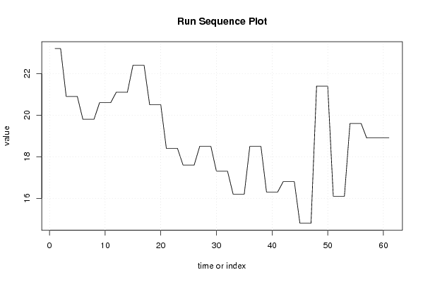
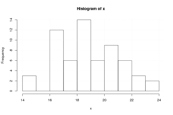
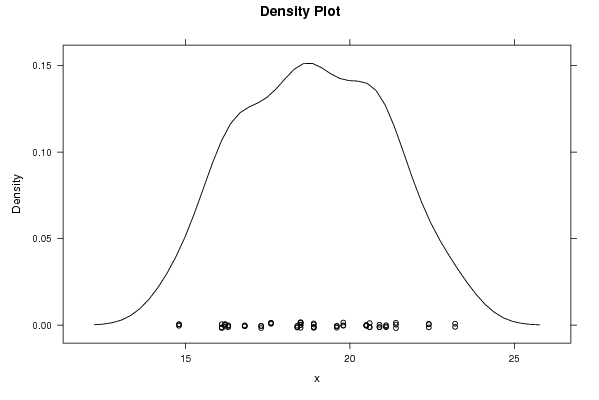
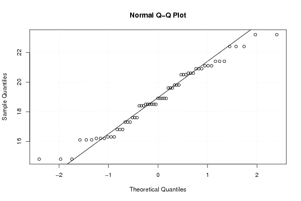
| Title produced by software | Univariate Explorative Data Analysis | ||||||||||||||||||||||||||||||||||||||||||||||||||||
| Date of computation | Fri, 18 Dec 2009 03:49:28 -0700 | ||||||||||||||||||||||||||||||||||||||||||||||||||||
| Cite this page as follows | Statistical Computations at FreeStatistics.org, Office for Research Development and Education, URL https://freestatistics.org/blog/index.php?v=date/2009/Dec/18/t1261133667il8cgk40l0yo24i.htm/, Retrieved Sat, 27 Apr 2024 11:27:54 +0000 | ||||||||||||||||||||||||||||||||||||||||||||||||||||
| Statistical Computations at FreeStatistics.org, Office for Research Development and Education, URL https://freestatistics.org/blog/index.php?pk=69224, Retrieved Sat, 27 Apr 2024 11:27:54 +0000 | |||||||||||||||||||||||||||||||||||||||||||||||||||||
| QR Codes: | |||||||||||||||||||||||||||||||||||||||||||||||||||||
|
| |||||||||||||||||||||||||||||||||||||||||||||||||||||
| Original text written by user: | |||||||||||||||||||||||||||||||||||||||||||||||||||||
| IsPrivate? | No (this computation is public) | ||||||||||||||||||||||||||||||||||||||||||||||||||||
| User-defined keywords | |||||||||||||||||||||||||||||||||||||||||||||||||||||
| Estimated Impact | 137 | ||||||||||||||||||||||||||||||||||||||||||||||||||||
Tree of Dependent Computations | |||||||||||||||||||||||||||||||||||||||||||||||||||||
| Family? (F = Feedback message, R = changed R code, M = changed R Module, P = changed Parameters, D = changed Data) | |||||||||||||||||||||||||||||||||||||||||||||||||||||
| - [Notched Boxplots] [3/11/2009] [2009-11-02 21:10:41] [b98453cac15ba1066b407e146608df68] - RMPD [Univariate Explorative Data Analysis] [Run sequence Omze...] [2009-11-05 09:18:51] [f5d341d4bbba73282fc6e80153a6d315] - [Univariate Explorative Data Analysis] [TG1] [2009-11-10 14:23:33] [a21bac9c8d3d56fdec8be4e719e2c7ed] - R [Univariate Explorative Data Analysis] [ws6] [2009-11-15 22:11:55] [3fc64fd7a52ce121dfe13dba27bf6e5b] - D [Univariate Explorative Data Analysis] [] [2009-12-18 10:22:11] [eea7474c6df699240a34279975905c82] - D [Univariate Explorative Data Analysis] [] [2009-12-18 10:49:28] [612b7913d2a3b4fa79d126829bd148db] [Current] | |||||||||||||||||||||||||||||||||||||||||||||||||||||
| Feedback Forum | |||||||||||||||||||||||||||||||||||||||||||||||||||||
Post a new message | |||||||||||||||||||||||||||||||||||||||||||||||||||||
Dataset | |||||||||||||||||||||||||||||||||||||||||||||||||||||
| Dataseries X: | |||||||||||||||||||||||||||||||||||||||||||||||||||||
23,2 23,2 20,9 20,9 20,9 19,8 19,8 19,8 20,6 20,6 20,6 21,1 21,1 21,1 22,4 22,4 22,4 20,5 20,5 20,5 18,4 18,4 18,4 17,6 17,6 17,6 18,5 18,5 18,5 17,3 17,3 17,3 16,2 16,2 16,2 18,5 18,5 18,5 16,3 16,3 16,3 16,8 16,8 16,8 14,8 14,8 14,8 21,4 21,4 21,4 16,1 16,1 16,1 19,6 19,6 19,6 18,9 18,9 18,9 18,9 18,9 | |||||||||||||||||||||||||||||||||||||||||||||||||||||
Tables (Output of Computation) | |||||||||||||||||||||||||||||||||||||||||||||||||||||
| |||||||||||||||||||||||||||||||||||||||||||||||||||||
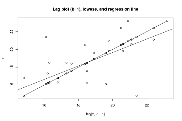
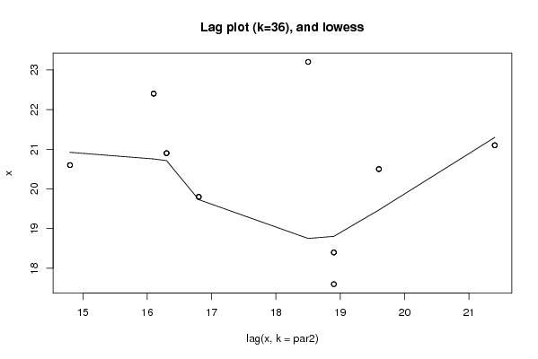
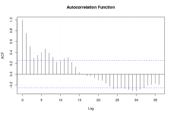
Figures (Output of Computation) | |||||||||||||||||||||||||||||||||||||||||||||||||||||
Input Parameters & R Code | |||||||||||||||||||||||||||||||||||||||||||||||||||||
| Parameters (Session): | |||||||||||||||||||||||||||||||||||||||||||||||||||||
| par1 = 0 ; par2 = 36 ; | |||||||||||||||||||||||||||||||||||||||||||||||||||||
| Parameters (R input): | |||||||||||||||||||||||||||||||||||||||||||||||||||||
| par1 = 0 ; par2 = 36 ; | |||||||||||||||||||||||||||||||||||||||||||||||||||||
| R code (references can be found in the software module): | |||||||||||||||||||||||||||||||||||||||||||||||||||||
par1 <- as.numeric(par1) | |||||||||||||||||||||||||||||||||||||||||||||||||||||