Repository of Reproducible Computations

Free Statistics

of Irreproducible Research!

Author's title

Author

*The author of this computation has been verified*

R Software Module

rwasp_arimaforecasting.wasp

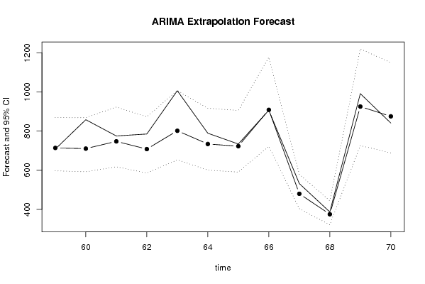
Title produced by software

ARIMA Forecasting

Date of computation

Fri, 18 Dec 2009 07:46:40 -0700

Cite this page as follows

Statistical Computations at FreeStatistics.org, Office for Research Development and Education, URL https://freestatistics.org/blog/index.php?v=date/2009/Dec/18/t12611477192n8jwo7kng989hi.htm/, Retrieved Sat, 27 Apr 2024 12:34:35 +0000

Statistical Computations at FreeStatistics.org, Office for Research Development and Education, URL https://freestatistics.org/blog/index.php?pk=69380, Retrieved Sat, 27 Apr 2024 12:34:35 +0000

QR Codes:

Paste this QR Code to cite your computation.

Original text written by user:

IsPrivate?

No (this computation is public)

User-defined keywords

Estimated Impact

142

Family? (F = Feedback message, R = changed R code, M = changed R Module, P = changed Parameters, D = changed Data)

-     [Standard Deviation-Mean Plot] [deel1 st dev mean...] [2009-12-16 19:13:20] [95cead3ebb75668735f848316249436a]
- RMP   [(Partial) Autocorrelation Function] [deel1 acf D=d=0] [2009-12-16 19:17:58] [95cead3ebb75668735f848316249436a]
-         [(Partial) Autocorrelation Function] [deel1 acf D=d=1] [2009-12-16 19:21:27] [95cead3ebb75668735f848316249436a]
- RM        [Variance Reduction Matrix] [deel1 vrm] [2009-12-16 19:23:09] [95cead3ebb75668735f848316249436a]
- RM          [Spectral Analysis] [deel1 spectrum D=d=1] [2009-12-16 19:31:03] [95cead3ebb75668735f848316249436a]
- RMP             [ARIMA Forecasting] [deel1 arima forca...] [2009-12-18 14:46:40] [95523ebdb89b97dbf680ec91e0b4bca2] [Current]
- RMPD              [Bivariate Granger Causality] [Granger Causality] [2009-12-19 17:16:50] [95cead3ebb75668735f848316249436a] 
-   P                 [Bivariate Granger Causality] [granger causality...] [2009-12-23 17:42:26] [95cead3ebb75668735f848316249436a] 
-                       [Bivariate Granger Causality] [Granger Causality...] [2009-12-23 18:23:32] [95cead3ebb75668735f848316249436a] 
-   P                     [Bivariate Granger Causality] [gr causality met ...] [2009-12-28 17:04:30] [95cead3ebb75668735f848316249436a] 
-   P                     [Bivariate Granger Causality] [gr causality met ...] [2009-12-28 17:09:15] [95cead3ebb75668735f848316249436a] 
-   P                     [Bivariate Granger Causality] [gr causality zond...] [2009-12-28 17:13:06] [95cead3ebb75668735f848316249436a] 
-   P                     [Bivariate Granger Causality] [gr causality zond...] [2009-12-28 17:14:47] [95cead3ebb75668735f848316249436a] 
-   P                     [Bivariate Granger Causality] [gr causality zond...] [2009-12-28 17:16:10] [95cead3ebb75668735f848316249436a] 
-   P                     [Bivariate Granger Causality] [gr causality zond...] [2009-12-28 17:18:27] [95cead3ebb75668735f848316249436a] 
-   P                     [Bivariate Granger Causality] [gr causality zond...] [2009-12-28 17:19:08] [95cead3ebb75668735f848316249436a] 
-   PD              [ARIMA Forecasting] [arima forecasting...] [2009-12-30 19:35:17] [acdebb2ecda2ddb208f4e14f4a68b9e7] 
-   P                 [ARIMA Forecasting] [forecasting (verk...] [2009-12-31 15:08:41] [acdebb2ecda2ddb208f4e14f4a68b9e7] 
-   PD              [ARIMA Forecasting] [Arima forecasting...] [2009-12-30 19:41:35] [acdebb2ecda2ddb208f4e14f4a68b9e7] 
-   PD              [ARIMA Forecasting] [forecast] [2009-12-31 15:49:20] [95cead3ebb75668735f848316249436a] 

Feedback Forum

Post a new message

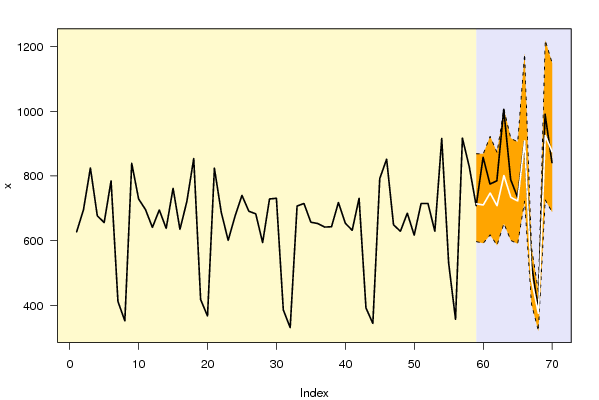
Dataseries X:

Download CSV

Histogram

Boxplots

Summary of computational transaction
Raw Input	view raw input (R code)
Raw Output	view raw output of R engine
Computing time	2 seconds
R Server	'Gwilym Jenkins' @ 72.249.127.135

\begin{tabular}{lllllllll}
\hline
Summary of computational transaction \tabularnewline
Raw Input & view raw input (R code)  \tabularnewline
Raw Output & view raw output of R engine  \tabularnewline
Computing time & 2 seconds \tabularnewline
R Server & 'Gwilym Jenkins' @ 72.249.127.135 \tabularnewline
\hline
\end{tabular}
%Source: https://freestatistics.org/blog/index.php?pk=69380&T=0

[TABLE]
[ROW][C]Summary of computational transaction[/C][/ROW]
[ROW][C]Raw Input[/C][C]view raw input (R code) [/C][/ROW]
[ROW][C]Raw Output[/C][C]view raw output of R engine [/C][/ROW]
[ROW][C]Computing time[/C][C]2 seconds[/C][/ROW]
[ROW][C]R Server[/C][C]'Gwilym Jenkins' @ 72.249.127.135[/C][/ROW]
[/TABLE]
Source: https://freestatistics.org/blog/index.php?pk=69380&T=0

Globally Unique Identifier (entire table): ba.freestatistics.org/blog/index.php?pk=69380&T=0

As an alternative you can also use a QR Code:

The GUIDs for individual cells are displayed in the table below:

Summary of computational transaction
Raw Input	view raw input (R code)
Raw Output	view raw output of R engine
Computing time	2 seconds
R Server	'Gwilym Jenkins' @ 72.249.127.135

Univariate ARIMA Extrapolation Forecast
time	Y[t]	F[t]	95% LB	95% UB	p-value(H0: Y[t] = F[t])	P(F[t]>Y[t-1])	P(F[t]>Y[t-s])	P(F[t]>Y[58])
46	852	-	-	-	-	-	-	-
47	649	-	-	-	-	-	-	-
48	629	-	-	-	-	-	-	-
49	685	-	-	-	-	-	-	-
50	617	-	-	-	-	-	-	-
51	715	-	-	-	-	-	-	-
52	715	-	-	-	-	-	-	-
53	629	-	-	-	-	-	-	-
54	916	-	-	-	-	-	-	-
55	531	-	-	-	-	-	-	-
56	357	-	-	-	-	-	-	-
57	917	-	-	-	-	-	-	-
58	828	-	-	-	-	-	-	-
59	708	713.8976	597.0477	868.7351	0.4702	0.0743	0.7943	0.0743
60	858	710.4361	592.029	868.2727	0.0334	0.5121	0.8441	0.0722
61	775	747.3977	617.7864	922.5263	0.3787	0.1079	0.7575	0.1835
62	785	707.9774	585.8363	872.7144	0.1797	0.2126	0.8605	0.0766
63	1006	801.5328	653.0875	1007.0026	0.0256	0.5627	0.7954	0.4003
64	789	733.9227	600.8368	916.6707	0.2774	0.0018	0.5804	0.1565
65	734	722.7877	590.4656	905.1368	0.452	0.2383	0.8433	0.1291
66	906	908.3614	722.2794	1176.8403	0.4931	0.8985	0.4778	0.7213
67	532	479.7532	403.9403	579.0989	0.1513	0	0.156	0
68	387	375.358	321.3396	444.2371	0.3702	0	0.6993	0
69	991	925.1193	725.8973	1219.2051	0.3303	0.9998	0.5216	0.7413
70	841	875.1282	688.545	1149.2634	0.4036	0.2037	0.6319	0.6319

\begin{tabular}{lllllllll}
\hline
Univariate ARIMA Extrapolation Forecast \tabularnewline
time & Y[t] & F[t] & 95% LB & 95% UB & p-value(H0: Y[t] = F[t]) & P(F[t]>Y[t-1]) & P(F[t]>Y[t-s]) & P(F[t]>Y[58]) \tabularnewline
46 & 852 & - & - & - & - & - & - & - \tabularnewline
47 & 649 & - & - & - & - & - & - & - \tabularnewline
48 & 629 & - & - & - & - & - & - & - \tabularnewline
49 & 685 & - & - & - & - & - & - & - \tabularnewline
50 & 617 & - & - & - & - & - & - & - \tabularnewline
51 & 715 & - & - & - & - & - & - & - \tabularnewline
52 & 715 & - & - & - & - & - & - & - \tabularnewline
53 & 629 & - & - & - & - & - & - & - \tabularnewline
54 & 916 & - & - & - & - & - & - & - \tabularnewline
55 & 531 & - & - & - & - & - & - & - \tabularnewline
56 & 357 & - & - & - & - & - & - & - \tabularnewline
57 & 917 & - & - & - & - & - & - & - \tabularnewline
58 & 828 & - & - & - & - & - & - & - \tabularnewline
59 & 708 & 713.8976 & 597.0477 & 868.7351 & 0.4702 & 0.0743 & 0.7943 & 0.0743 \tabularnewline
60 & 858 & 710.4361 & 592.029 & 868.2727 & 0.0334 & 0.5121 & 0.8441 & 0.0722 \tabularnewline
61 & 775 & 747.3977 & 617.7864 & 922.5263 & 0.3787 & 0.1079 & 0.7575 & 0.1835 \tabularnewline
62 & 785 & 707.9774 & 585.8363 & 872.7144 & 0.1797 & 0.2126 & 0.8605 & 0.0766 \tabularnewline
63 & 1006 & 801.5328 & 653.0875 & 1007.0026 & 0.0256 & 0.5627 & 0.7954 & 0.4003 \tabularnewline
64 & 789 & 733.9227 & 600.8368 & 916.6707 & 0.2774 & 0.0018 & 0.5804 & 0.1565 \tabularnewline
65 & 734 & 722.7877 & 590.4656 & 905.1368 & 0.452 & 0.2383 & 0.8433 & 0.1291 \tabularnewline
66 & 906 & 908.3614 & 722.2794 & 1176.8403 & 0.4931 & 0.8985 & 0.4778 & 0.7213 \tabularnewline
67 & 532 & 479.7532 & 403.9403 & 579.0989 & 0.1513 & 0 & 0.156 & 0 \tabularnewline
68 & 387 & 375.358 & 321.3396 & 444.2371 & 0.3702 & 0 & 0.6993 & 0 \tabularnewline
69 & 991 & 925.1193 & 725.8973 & 1219.2051 & 0.3303 & 0.9998 & 0.5216 & 0.7413 \tabularnewline
70 & 841 & 875.1282 & 688.545 & 1149.2634 & 0.4036 & 0.2037 & 0.6319 & 0.6319 \tabularnewline
\hline
\end{tabular}
%Source: https://freestatistics.org/blog/index.php?pk=69380&T=1

[TABLE]
[ROW][C]Univariate ARIMA Extrapolation Forecast[/C][/ROW]
[ROW][C]time[/C][C]Y[t][/C][C]F[t][/C][C]95% LB[/C][C]95% UB[/C][C]p-value(H0: Y[t] = F[t])[/C][C]P(F[t]>Y[t-1])[/C][C]P(F[t]>Y[t-s])[/C][C]P(F[t]>Y[58])[/C][/ROW]
[ROW][C]46[/C][C]852[/C][C]-[/C][C]-[/C][C]-[/C][C]-[/C][C]-[/C][C]-[/C][C]-[/C][/ROW]
[ROW][C]47[/C][C]649[/C][C]-[/C][C]-[/C][C]-[/C][C]-[/C][C]-[/C][C]-[/C][C]-[/C][/ROW]
[ROW][C]48[/C][C]629[/C][C]-[/C][C]-[/C][C]-[/C][C]-[/C][C]-[/C][C]-[/C][C]-[/C][/ROW]
[ROW][C]49[/C][C]685[/C][C]-[/C][C]-[/C][C]-[/C][C]-[/C][C]-[/C][C]-[/C][C]-[/C][/ROW]
[ROW][C]50[/C][C]617[/C][C]-[/C][C]-[/C][C]-[/C][C]-[/C][C]-[/C][C]-[/C][C]-[/C][/ROW]
[ROW][C]51[/C][C]715[/C][C]-[/C][C]-[/C][C]-[/C][C]-[/C][C]-[/C][C]-[/C][C]-[/C][/ROW]
[ROW][C]52[/C][C]715[/C][C]-[/C][C]-[/C][C]-[/C][C]-[/C][C]-[/C][C]-[/C][C]-[/C][/ROW]
[ROW][C]53[/C][C]629[/C][C]-[/C][C]-[/C][C]-[/C][C]-[/C][C]-[/C][C]-[/C][C]-[/C][/ROW]
[ROW][C]54[/C][C]916[/C][C]-[/C][C]-[/C][C]-[/C][C]-[/C][C]-[/C][C]-[/C][C]-[/C][/ROW]
[ROW][C]55[/C][C]531[/C][C]-[/C][C]-[/C][C]-[/C][C]-[/C][C]-[/C][C]-[/C][C]-[/C][/ROW]
[ROW][C]56[/C][C]357[/C][C]-[/C][C]-[/C][C]-[/C][C]-[/C][C]-[/C][C]-[/C][C]-[/C][/ROW]
[ROW][C]57[/C][C]917[/C][C]-[/C][C]-[/C][C]-[/C][C]-[/C][C]-[/C][C]-[/C][C]-[/C][/ROW]
[ROW][C]58[/C][C]828[/C][C]-[/C][C]-[/C][C]-[/C][C]-[/C][C]-[/C][C]-[/C][C]-[/C][/ROW]
[ROW][C]59[/C][C]708[/C][C]713.8976[/C][C]597.0477[/C][C]868.7351[/C][C]0.4702[/C][C]0.0743[/C][C]0.7943[/C][C]0.0743[/C][/ROW]
[ROW][C]60[/C][C]858[/C][C]710.4361[/C][C]592.029[/C][C]868.2727[/C][C]0.0334[/C][C]0.5121[/C][C]0.8441[/C][C]0.0722[/C][/ROW]
[ROW][C]61[/C][C]775[/C][C]747.3977[/C][C]617.7864[/C][C]922.5263[/C][C]0.3787[/C][C]0.1079[/C][C]0.7575[/C][C]0.1835[/C][/ROW]
[ROW][C]62[/C][C]785[/C][C]707.9774[/C][C]585.8363[/C][C]872.7144[/C][C]0.1797[/C][C]0.2126[/C][C]0.8605[/C][C]0.0766[/C][/ROW]
[ROW][C]63[/C][C]1006[/C][C]801.5328[/C][C]653.0875[/C][C]1007.0026[/C][C]0.0256[/C][C]0.5627[/C][C]0.7954[/C][C]0.4003[/C][/ROW]
[ROW][C]64[/C][C]789[/C][C]733.9227[/C][C]600.8368[/C][C]916.6707[/C][C]0.2774[/C][C]0.0018[/C][C]0.5804[/C][C]0.1565[/C][/ROW]
[ROW][C]65[/C][C]734[/C][C]722.7877[/C][C]590.4656[/C][C]905.1368[/C][C]0.452[/C][C]0.2383[/C][C]0.8433[/C][C]0.1291[/C][/ROW]
[ROW][C]66[/C][C]906[/C][C]908.3614[/C][C]722.2794[/C][C]1176.8403[/C][C]0.4931[/C][C]0.8985[/C][C]0.4778[/C][C]0.7213[/C][/ROW]
[ROW][C]67[/C][C]532[/C][C]479.7532[/C][C]403.9403[/C][C]579.0989[/C][C]0.1513[/C][C]0[/C][C]0.156[/C][C]0[/C][/ROW]
[ROW][C]68[/C][C]387[/C][C]375.358[/C][C]321.3396[/C][C]444.2371[/C][C]0.3702[/C][C]0[/C][C]0.6993[/C][C]0[/C][/ROW]
[ROW][C]69[/C][C]991[/C][C]925.1193[/C][C]725.8973[/C][C]1219.2051[/C][C]0.3303[/C][C]0.9998[/C][C]0.5216[/C][C]0.7413[/C][/ROW]
[ROW][C]70[/C][C]841[/C][C]875.1282[/C][C]688.545[/C][C]1149.2634[/C][C]0.4036[/C][C]0.2037[/C][C]0.6319[/C][C]0.6319[/C][/ROW]
[/TABLE]
Source: https://freestatistics.org/blog/index.php?pk=69380&T=1

Globally Unique Identifier (entire table): ba.freestatistics.org/blog/index.php?pk=69380&T=1

As an alternative you can also use a QR Code:

The GUIDs for individual cells are displayed in the table below:

Univariate ARIMA Extrapolation Forecast
time	Y[t]	F[t]	95% LB	95% UB	p-value(H0: Y[t] = F[t])	P(F[t]>Y[t-1])	P(F[t]>Y[t-s])	P(F[t]>Y[58])
46	852	-	-	-	-	-	-	-
47	649	-	-	-	-	-	-	-
48	629	-	-	-	-	-	-	-
49	685	-	-	-	-	-	-	-
50	617	-	-	-	-	-	-	-
51	715	-	-	-	-	-	-	-
52	715	-	-	-	-	-	-	-
53	629	-	-	-	-	-	-	-
54	916	-	-	-	-	-	-	-
55	531	-	-	-	-	-	-	-
56	357	-	-	-	-	-	-	-
57	917	-	-	-	-	-	-	-
58	828	-	-	-	-	-	-	-
59	708	713.8976	597.0477	868.7351	0.4702	0.0743	0.7943	0.0743
60	858	710.4361	592.029	868.2727	0.0334	0.5121	0.8441	0.0722
61	775	747.3977	617.7864	922.5263	0.3787	0.1079	0.7575	0.1835
62	785	707.9774	585.8363	872.7144	0.1797	0.2126	0.8605	0.0766
63	1006	801.5328	653.0875	1007.0026	0.0256	0.5627	0.7954	0.4003
64	789	733.9227	600.8368	916.6707	0.2774	0.0018	0.5804	0.1565
65	734	722.7877	590.4656	905.1368	0.452	0.2383	0.8433	0.1291
66	906	908.3614	722.2794	1176.8403	0.4931	0.8985	0.4778	0.7213
67	532	479.7532	403.9403	579.0989	0.1513	0	0.156	0
68	387	375.358	321.3396	444.2371	0.3702	0	0.6993	0
69	991	925.1193	725.8973	1219.2051	0.3303	0.9998	0.5216	0.7413
70	841	875.1282	688.545	1149.2634	0.4036	0.2037	0.6319	0.6319

Univariate ARIMA Extrapolation Forecast Performance
time	% S.E.	PE	MAPE	Sq.E	MSE	RMSE
59	0.1107	-0.0083	0	34.7814	0	0
60	0.1134	0.2077	0.108	21775.1019	10904.9416	104.4267
61	0.1195	0.0369	0.0843	761.8873	7523.9235	86.7406
62	0.1187	0.1088	0.0904	5932.4779	7126.0621	84.416
63	0.1308	0.2551	0.1234	41806.8403	14062.2177	118.5842
64	0.127	0.075	0.1153	3033.504	12224.0988	110.5626
65	0.1287	0.0155	0.101	125.7164	10495.7585	102.4488
66	0.1508	-0.0026	0.0887	5.576	9184.4856	95.8357
67	0.1057	0.1089	0.091	2729.7248	8467.29	92.0179
68	0.0936	0.031	0.085	135.5354	7634.1145	87.3734
69	0.1622	0.0712	0.0837	4340.2648	7334.6737	85.6427
70	0.1598	-0.039	0.08	1164.7311	6820.5118	82.5864

\begin{tabular}{lllllllll}
\hline
Univariate ARIMA Extrapolation Forecast Performance \tabularnewline
time & % S.E. & PE & MAPE & Sq.E & MSE & RMSE \tabularnewline
59 & 0.1107 & -0.0083 & 0 & 34.7814 & 0 & 0 \tabularnewline
60 & 0.1134 & 0.2077 & 0.108 & 21775.1019 & 10904.9416 & 104.4267 \tabularnewline
61 & 0.1195 & 0.0369 & 0.0843 & 761.8873 & 7523.9235 & 86.7406 \tabularnewline
62 & 0.1187 & 0.1088 & 0.0904 & 5932.4779 & 7126.0621 & 84.416 \tabularnewline
63 & 0.1308 & 0.2551 & 0.1234 & 41806.8403 & 14062.2177 & 118.5842 \tabularnewline
64 & 0.127 & 0.075 & 0.1153 & 3033.504 & 12224.0988 & 110.5626 \tabularnewline
65 & 0.1287 & 0.0155 & 0.101 & 125.7164 & 10495.7585 & 102.4488 \tabularnewline
66 & 0.1508 & -0.0026 & 0.0887 & 5.576 & 9184.4856 & 95.8357 \tabularnewline
67 & 0.1057 & 0.1089 & 0.091 & 2729.7248 & 8467.29 & 92.0179 \tabularnewline
68 & 0.0936 & 0.031 & 0.085 & 135.5354 & 7634.1145 & 87.3734 \tabularnewline
69 & 0.1622 & 0.0712 & 0.0837 & 4340.2648 & 7334.6737 & 85.6427 \tabularnewline
70 & 0.1598 & -0.039 & 0.08 & 1164.7311 & 6820.5118 & 82.5864 \tabularnewline
\hline
\end{tabular}
%Source: https://freestatistics.org/blog/index.php?pk=69380&T=2

[TABLE]
[ROW][C]Univariate ARIMA Extrapolation Forecast Performance[/C][/ROW]
[ROW][C]time[/C][C]% S.E.[/C][C]PE[/C][C]MAPE[/C][C]Sq.E[/C][C]MSE[/C][C]RMSE[/C][/ROW]
[ROW][C]59[/C][C]0.1107[/C][C]-0.0083[/C][C]0[/C][C]34.7814[/C][C]0[/C][C]0[/C][/ROW]
[ROW][C]60[/C][C]0.1134[/C][C]0.2077[/C][C]0.108[/C][C]21775.1019[/C][C]10904.9416[/C][C]104.4267[/C][/ROW]
[ROW][C]61[/C][C]0.1195[/C][C]0.0369[/C][C]0.0843[/C][C]761.8873[/C][C]7523.9235[/C][C]86.7406[/C][/ROW]
[ROW][C]62[/C][C]0.1187[/C][C]0.1088[/C][C]0.0904[/C][C]5932.4779[/C][C]7126.0621[/C][C]84.416[/C][/ROW]
[ROW][C]63[/C][C]0.1308[/C][C]0.2551[/C][C]0.1234[/C][C]41806.8403[/C][C]14062.2177[/C][C]118.5842[/C][/ROW]
[ROW][C]64[/C][C]0.127[/C][C]0.075[/C][C]0.1153[/C][C]3033.504[/C][C]12224.0988[/C][C]110.5626[/C][/ROW]
[ROW][C]65[/C][C]0.1287[/C][C]0.0155[/C][C]0.101[/C][C]125.7164[/C][C]10495.7585[/C][C]102.4488[/C][/ROW]
[ROW][C]66[/C][C]0.1508[/C][C]-0.0026[/C][C]0.0887[/C][C]5.576[/C][C]9184.4856[/C][C]95.8357[/C][/ROW]
[ROW][C]67[/C][C]0.1057[/C][C]0.1089[/C][C]0.091[/C][C]2729.7248[/C][C]8467.29[/C][C]92.0179[/C][/ROW]
[ROW][C]68[/C][C]0.0936[/C][C]0.031[/C][C]0.085[/C][C]135.5354[/C][C]7634.1145[/C][C]87.3734[/C][/ROW]
[ROW][C]69[/C][C]0.1622[/C][C]0.0712[/C][C]0.0837[/C][C]4340.2648[/C][C]7334.6737[/C][C]85.6427[/C][/ROW]
[ROW][C]70[/C][C]0.1598[/C][C]-0.039[/C][C]0.08[/C][C]1164.7311[/C][C]6820.5118[/C][C]82.5864[/C][/ROW]
[/TABLE]
Source: https://freestatistics.org/blog/index.php?pk=69380&T=2

Globally Unique Identifier (entire table): ba.freestatistics.org/blog/index.php?pk=69380&T=2

As an alternative you can also use a QR Code:

The GUIDs for individual cells are displayed in the table below:

Univariate ARIMA Extrapolation Forecast Performance
time	% S.E.	PE	MAPE	Sq.E	MSE	RMSE
59	0.1107	-0.0083	0	34.7814	0	0
60	0.1134	0.2077	0.108	21775.1019	10904.9416	104.4267
61	0.1195	0.0369	0.0843	761.8873	7523.9235	86.7406
62	0.1187	0.1088	0.0904	5932.4779	7126.0621	84.416
63	0.1308	0.2551	0.1234	41806.8403	14062.2177	118.5842
64	0.127	0.075	0.1153	3033.504	12224.0988	110.5626
65	0.1287	0.0155	0.101	125.7164	10495.7585	102.4488
66	0.1508	-0.0026	0.0887	5.576	9184.4856	95.8357
67	0.1057	0.1089	0.091	2729.7248	8467.29	92.0179
68	0.0936	0.031	0.085	135.5354	7634.1145	87.3734
69	0.1622	0.0712	0.0837	4340.2648	7334.6737	85.6427
70	0.1598	-0.039	0.08	1164.7311	6820.5118	82.5864

Figure 1

PNG link

Postscript link

PDF link

Figure 2

PNG link

Postscript link

PDF link

Parameters (Session):

par1 = TRUE ; par2 = -0.5 ; par3 = 1 ; par4 = 1 ; par5 = 12 ; par6 = 3 ; par7 = 1 ; par8 = 2 ; par9 = 0 ;

Parameters (R input):

par1 = 12 ; par2 = -0.5 ; par3 = 1 ; par4 = 1 ; par5 = 12 ; par6 = 0 ; par7 = 1 ; par8 = 0 ; par9 = 1 ; par10 = FALSE ;

R code (references can be found in the software module):

par1 <- as.numeric(par1) #cut off periods
par2 <- as.numeric(par2) #lambda
par3 <- as.numeric(par3) #degree of non-seasonal differencing
par4 <- as.numeric(par4) #degree of seasonal differencing
par5 <- as.numeric(par5) #seasonal period
par6 <- as.numeric(par6) #p
par7 <- as.numeric(par7) #q
par8 <- as.numeric(par8) #P
par9 <- as.numeric(par9) #Q
if (par10 == 'TRUE') par10 <- TRUE
if (par10 == 'FALSE') par10 <- FALSE
if (par2 == 0) x <- log(x)
if (par2 != 0) x <- x^par2
lx <- length(x)
first <- lx - 2*par1
nx <- lx - par1
nx1 <- nx + 1
fx <- lx - nx
if (fx < 1) {
fx <- par5
nx1 <- lx + fx - 1
first <- lx - 2*fx
}
first <- 1
if (fx < 3) fx <- round(lx/10,0)
(arima.out <- arima(x[1:nx], order=c(par6,par3,par7), seasonal=list(order=c(par8,par4,par9), period=par5), include.mean=par10, method='ML'))
(forecast <- predict(arima.out,par1))
(lb <- forecast$pred - 1.96 * forecast$se)
(ub <- forecast$pred + 1.96 * forecast$se)
if (par2 == 0) {
x <- exp(x)
forecast$pred <- exp(forecast$pred)
lb <- exp(lb)
ub <- exp(ub)
}
if (par2 != 0) {
x <- x^(1/par2)
forecast$pred <- forecast$pred^(1/par2)
lb <- lb^(1/par2)
ub <- ub^(1/par2)
}
if (par2 < 0) {
olb <- lb
lb <- ub
ub <- olb
}
(actandfor <- c(x[1:nx], forecast$pred))
(perc.se <- (ub-forecast$pred)/1.96/forecast$pred)
bitmap(file='test1.png')
opar <- par(mar=c(4,4,2,2),las=1)
ylim <- c( min(x[first:nx],lb), max(x[first:nx],ub))
plot(x,ylim=ylim,type='n',xlim=c(first,lx))
usr <- par('usr')
rect(usr[1],usr[3],nx+1,usr[4],border=NA,col='lemonchiffon')
rect(nx1,usr[3],usr[2],usr[4],border=NA,col='lavender')
abline(h= (-3:3)*2 , col ='gray', lty =3)
polygon( c(nx1:lx,lx:nx1), c(lb,rev(ub)), col = 'orange', lty=2,border=NA)
lines(nx1:lx, lb , lty=2)
lines(nx1:lx, ub , lty=2)
lines(x, lwd=2)
lines(nx1:lx, forecast$pred , lwd=2 , col ='white')
box()
par(opar)
dev.off()
prob.dec <- array(NA, dim=fx)
prob.sdec <- array(NA, dim=fx)
prob.ldec <- array(NA, dim=fx)
prob.pval <- array(NA, dim=fx)
perf.pe <- array(0, dim=fx)
perf.mape <- array(0, dim=fx)
perf.mape1 <- array(0, dim=fx)
perf.se <- array(0, dim=fx)
perf.mse <- array(0, dim=fx)
perf.mse1 <- array(0, dim=fx)
perf.rmse <- array(0, dim=fx)
for (i in 1:fx) {
locSD <- (ub[i] - forecast$pred[i]) / 1.96
perf.pe[i] = (x[nx+i] - forecast$pred[i]) / forecast$pred[i]
perf.se[i] = (x[nx+i] - forecast$pred[i])^2
prob.dec[i] = pnorm((x[nx+i-1] - forecast$pred[i]) / locSD)
prob.sdec[i] = pnorm((x[nx+i-par5] - forecast$pred[i]) / locSD)
prob.ldec[i] = pnorm((x[nx] - forecast$pred[i]) / locSD)
prob.pval[i] = pnorm(abs(x[nx+i] - forecast$pred[i]) / locSD)
}
perf.mape[1] = abs(perf.pe[1])
perf.mse[1] = abs(perf.se[1])
for (i in 2:fx) {
perf.mape[i] = perf.mape[i-1] + abs(perf.pe[i])
perf.mape1[i] = perf.mape[i] / i
perf.mse[i] = perf.mse[i-1] + perf.se[i]
perf.mse1[i] = perf.mse[i] / i
}
perf.rmse = sqrt(perf.mse1)
bitmap(file='test2.png')
plot(forecast$pred, pch=19, type='b',main='ARIMA Extrapolation Forecast', ylab='Forecast and 95% CI', xlab='time',ylim=c(min(lb),max(ub)))
dum <- forecast$pred
dum[1:par1] <- x[(nx+1):lx]
lines(dum, lty=1)
lines(ub,lty=3)
lines(lb,lty=3)
dev.off()
load(file='createtable')
a<-table.start()
a<-table.row.start(a)
a<-table.element(a,'Univariate ARIMA Extrapolation Forecast',9,TRUE)
a<-table.row.end(a)
a<-table.row.start(a)
a<-table.element(a,'time',1,header=TRUE)
a<-table.element(a,'Y[t]',1,header=TRUE)
a<-table.element(a,'F[t]',1,header=TRUE)
a<-table.element(a,'95% LB',1,header=TRUE)
a<-table.element(a,'95% UB',1,header=TRUE)
a<-table.element(a,'p-value
(H0: Y[t] = F[t])',1,header=TRUE)
a<-table.element(a,'P(F[t]>Y[t-1])',1,header=TRUE)
a<-table.element(a,'P(F[t]>Y[t-s])',1,header=TRUE)
mylab <- paste('P(F[t]>Y[',nx,sep='')
mylab <- paste(mylab,'])',sep='')
a<-table.element(a,mylab,1,header=TRUE)
a<-table.row.end(a)
for (i in (nx-par5):nx) {
a<-table.row.start(a)
a<-table.element(a,i,header=TRUE)
a<-table.element(a,x[i])
a<-table.element(a,'-')
a<-table.element(a,'-')
a<-table.element(a,'-')
a<-table.element(a,'-')
a<-table.element(a,'-')
a<-table.element(a,'-')
a<-table.element(a,'-')
a<-table.row.end(a)
}
for (i in 1:fx) {
a<-table.row.start(a)
a<-table.element(a,nx+i,header=TRUE)
a<-table.element(a,round(x[nx+i],4))
a<-table.element(a,round(forecast$pred[i],4))
a<-table.element(a,round(lb[i],4))
a<-table.element(a,round(ub[i],4))
a<-table.element(a,round((1-prob.pval[i]),4))
a<-table.element(a,round((1-prob.dec[i]),4))
a<-table.element(a,round((1-prob.sdec[i]),4))
a<-table.element(a,round((1-prob.ldec[i]),4))
a<-table.row.end(a)
}
a<-table.end(a)
table.save(a,file='mytable.tab')
a<-table.start()
a<-table.row.start(a)
a<-table.element(a,'Univariate ARIMA Extrapolation Forecast Performance',7,TRUE)
a<-table.row.end(a)
a<-table.row.start(a)
a<-table.element(a,'time',1,header=TRUE)
a<-table.element(a,'% S.E.',1,header=TRUE)
a<-table.element(a,'PE',1,header=TRUE)
a<-table.element(a,'MAPE',1,header=TRUE)
a<-table.element(a,'Sq.E',1,header=TRUE)
a<-table.element(a,'MSE',1,header=TRUE)
a<-table.element(a,'RMSE',1,header=TRUE)
a<-table.row.end(a)
for (i in 1:fx) {
a<-table.row.start(a)
a<-table.element(a,nx+i,header=TRUE)
a<-table.element(a,round(perc.se[i],4))
a<-table.element(a,round(perf.pe[i],4))
a<-table.element(a,round(perf.mape1[i],4))
a<-table.element(a,round(perf.se[i],4))
a<-table.element(a,round(perf.mse1[i],4))
a<-table.element(a,round(perf.rmse[i],4))
a<-table.row.end(a)
}
a<-table.end(a)
table.save(a,file='mytable1.tab')

Free Statistics

Description of Statistical Computation

Tree of Dependent Computations

Dataset

Tables (Output of Computation)

Figures (Output of Computation)

Input Parameters & R Code