Free Statistics
of Irreproducible Research!
Description of Statistical Computation | |||||||||||||||||||||||||||||||||||||||||||||
|---|---|---|---|---|---|---|---|---|---|---|---|---|---|---|---|---|---|---|---|---|---|---|---|---|---|---|---|---|---|---|---|---|---|---|---|---|---|---|---|---|---|---|---|---|---|
| Author's title | |||||||||||||||||||||||||||||||||||||||||||||
| Author | *The author of this computation has been verified* | ||||||||||||||||||||||||||||||||||||||||||||
| R Software Module | rwasp_boxcoxlin.wasp | ||||||||||||||||||||||||||||||||||||||||||||
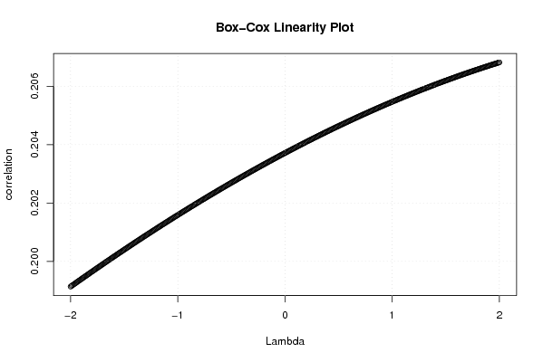
| Title produced by software | Box-Cox Linearity Plot | ||||||||||||||||||||||||||||||||||||||||||||
| Date of computation | Fri, 18 Dec 2009 07:48:55 -0700 | ||||||||||||||||||||||||||||||||||||||||||||
| Cite this page as follows | Statistical Computations at FreeStatistics.org, Office for Research Development and Education, URL https://freestatistics.org/blog/index.php?v=date/2009/Dec/18/t1261147846kevzsmx29n3dnrv.htm/, Retrieved Sat, 27 Apr 2024 09:43:05 +0000 | ||||||||||||||||||||||||||||||||||||||||||||
| Statistical Computations at FreeStatistics.org, Office for Research Development and Education, URL https://freestatistics.org/blog/index.php?pk=69382, Retrieved Sat, 27 Apr 2024 09:43:05 +0000 | |||||||||||||||||||||||||||||||||||||||||||||
| QR Codes: | |||||||||||||||||||||||||||||||||||||||||||||
|
| |||||||||||||||||||||||||||||||||||||||||||||
| Original text written by user: | |||||||||||||||||||||||||||||||||||||||||||||
| IsPrivate? | No (this computation is public) | ||||||||||||||||||||||||||||||||||||||||||||
| User-defined keywords | SHW Paper: Box-Cox linearity plot | ||||||||||||||||||||||||||||||||||||||||||||
| Estimated Impact | 134 | ||||||||||||||||||||||||||||||||||||||||||||
Tree of Dependent Computations | |||||||||||||||||||||||||||||||||||||||||||||
| Family? (F = Feedback message, R = changed R code, M = changed R Module, P = changed Parameters, D = changed Data) | |||||||||||||||||||||||||||||||||||||||||||||
| - [Box-Cox Linearity Plot] [3/11/2009] [2009-11-02 21:47:57] [b98453cac15ba1066b407e146608df68] - D [Box-Cox Linearity Plot] [WS 6 Box-Cox Line...] [2009-11-05 10:35:46] [b103a1dc147def8132c7f643ad8c8f84] - D [Box-Cox Linearity Plot] [Paper: Box-Cox li...] [2009-12-17 12:28:42] [b103a1dc147def8132c7f643ad8c8f84] - R [Box-Cox Linearity Plot] [] [2009-12-18 09:15:07] [b98453cac15ba1066b407e146608df68] - [Box-Cox Linearity Plot] [Paper: Box-Cox li...] [2009-12-18 14:48:55] [a45cc820faa25ce30779915639528ec2] [Current] | |||||||||||||||||||||||||||||||||||||||||||||
| Feedback Forum | |||||||||||||||||||||||||||||||||||||||||||||
Post a new message | |||||||||||||||||||||||||||||||||||||||||||||
Dataset | |||||||||||||||||||||||||||||||||||||||||||||
| Dataseries X: | |||||||||||||||||||||||||||||||||||||||||||||
-0.8 -0.2 0.2 1 0 -0.2 1 0.4 1 1.7 3.1 3.3 3.1 3.5 6 5.7 4.7 4.2 3.6 4.4 2.5 -0.6 -1.9 -1.9 0.7 -0.9 -1.7 -3.1 -2.1 0.2 1.2 3.8 4 6.6 5.3 7.6 4.7 6.6 4.4 4.6 6 4.8 4 2.7 3 4.1 4 2.7 2.6 3.1 4.4 3 2 1.3 1.5 1.3 3.2 1.8 3.3 1 2.4 0.4 -0.1 1.3 -1.1 -4.4 -7.5 -12.2 -14.5 -16 -16.7 -16.3 -16.9 | |||||||||||||||||||||||||||||||||||||||||||||
| Dataseries Y: | |||||||||||||||||||||||||||||||||||||||||||||
15.5 15.1 11.7 16.3 16.7 15 14.9 14.6 15.3 17.9 16.4 15.4 17.9 15.9 13.9 17.8 17.9 17.4 16.7 16 16.6 19.1 17.8 17.2 18.6 16.3 15.1 19.2 17.7 19.1 18 17.5 17.8 21.1 17.2 19.4 19.8 17.6 16.2 19.5 19.9 20 17.3 18.9 18.6 21.4 18.6 19.8 20.8 19.6 17.7 19.8 22.2 20.7 17.9 20.9 21.2 21.4 23 21.3 23.9 22.4 18.3 22.8 22.3 17.8 16.4 16 16.4 17.7 16.6 16.2 18.3 | |||||||||||||||||||||||||||||||||||||||||||||
Tables (Output of Computation) | |||||||||||||||||||||||||||||||||||||||||||||
| |||||||||||||||||||||||||||||||||||||||||||||
Figures (Output of Computation) | |||||||||||||||||||||||||||||||||||||||||||||
Input Parameters & R Code | |||||||||||||||||||||||||||||||||||||||||||||
| Parameters (Session): | |||||||||||||||||||||||||||||||||||||||||||||
| Parameters (R input): | |||||||||||||||||||||||||||||||||||||||||||||
| par1 = ; par2 = ; par3 = ; par4 = ; par5 = ; par6 = ; par7 = ; par8 = ; par9 = ; par10 = ; par11 = ; par12 = ; par13 = ; par14 = ; par15 = ; par16 = ; par17 = ; par18 = ; par19 = ; par20 = ; | |||||||||||||||||||||||||||||||||||||||||||||
| R code (references can be found in the software module): | |||||||||||||||||||||||||||||||||||||||||||||
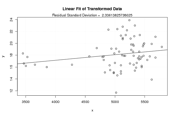
x <- x +100 | |||||||||||||||||||||||||||||||||||||||||||||