Repository of Reproducible Computations

Free Statistics

of Irreproducible Research!

Author's title

Author

*The author of this computation has been verified*

R Software Module

rwasp_autocorrelation.wasp

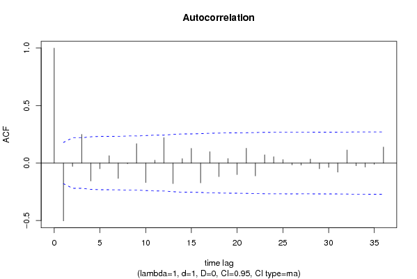
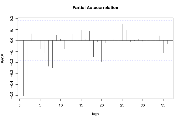
Title produced by software

(Partial) Autocorrelation Function

Date of computation

Sun, 20 Dec 2009 11:41:02 -0700

Cite this page as follows

Statistical Computations at FreeStatistics.org, Office for Research Development and Education, URL https://freestatistics.org/blog/index.php?v=date/2009/Dec/20/t1261334512yfuryvlvno6lnuq.htm/, Retrieved Sat, 27 Apr 2024 12:03:07 +0000

Statistical Computations at FreeStatistics.org, Office for Research Development and Education, URL https://freestatistics.org/blog/index.php?pk=69979, Retrieved Sat, 27 Apr 2024 12:03:07 +0000

QR Codes:

Paste this QR Code to cite your computation.

Original text written by user:

IsPrivate?

No (this computation is public)

User-defined keywords

Estimated Impact

144

Family? (F = Feedback message, R = changed R code, M = changed R Module, P = changed Parameters, D = changed Data)

-     [Univariate Data Series] [data set] [2008-12-01 19:54:57] [b98453cac15ba1066b407e146608df68]
- RMP   [(Partial) Autocorrelation Function] [] [2009-11-27 14:48:46] [b98453cac15ba1066b407e146608df68]
-   PD    [(Partial) Autocorrelation Function] [ACF (d = 2, D = 1)] [2009-12-02 16:44:37] [ee7c2e7343f5b1451e62c5c16ec521f1]
-   P       [(Partial) Autocorrelation Function] [ACF (d = 1, D = 0)] [2009-12-02 19:32:48] [ee7c2e7343f5b1451e62c5c16ec521f1]
-             [(Partial) Autocorrelation Function] [] [2009-12-04 21:31:38] [859f65298c93b90426725427c75f8582]
-    D            [(Partial) Autocorrelation Function] [] [2009-12-20 18:41:02] [d5175f34d1f80375edd7cbd8232724fe] [Current]

Feedback Forum

Post a new message

Dataseries X:

Download CSV

Histogram

Boxplots

Summary of computational transaction
Raw Input	view raw input (R code)
Raw Output	view raw output of R engine
Computing time	1 seconds
R Server	'Gwilym Jenkins' @ 72.249.127.135

\begin{tabular}{lllllllll}
\hline
Summary of computational transaction \tabularnewline
Raw Input & view raw input (R code)  \tabularnewline
Raw Output & view raw output of R engine  \tabularnewline
Computing time & 1 seconds \tabularnewline
R Server & 'Gwilym Jenkins' @ 72.249.127.135 \tabularnewline
\hline
\end{tabular}
%Source: https://freestatistics.org/blog/index.php?pk=69979&T=0

[TABLE]
[ROW][C]Summary of computational transaction[/C][/ROW]
[ROW][C]Raw Input[/C][C]view raw input (R code) [/C][/ROW]
[ROW][C]Raw Output[/C][C]view raw output of R engine [/C][/ROW]
[ROW][C]Computing time[/C][C]1 seconds[/C][/ROW]
[ROW][C]R Server[/C][C]'Gwilym Jenkins' @ 72.249.127.135[/C][/ROW]
[/TABLE]
Source: https://freestatistics.org/blog/index.php?pk=69979&T=0

Globally Unique Identifier (entire table): ba.freestatistics.org/blog/index.php?pk=69979&T=0

As an alternative you can also use a QR Code:

The GUIDs for individual cells are displayed in the table below:

Summary of computational transaction
Raw Input	view raw input (R code)
Raw Output	view raw output of R engine
Computing time	1 seconds
R Server	'Gwilym Jenkins' @ 72.249.127.135

Autocorrelation Function
Time lag k	ACF(k)	T-STAT	P-value
1	-0.502888	-5.5089	0
2	-0.02897	-0.3174	0.375764
3	0.24951	2.7333	0.00361
4	-0.156472	-1.7141	0.04455
5	-0.049559	-0.5429	0.294106
6	0.064173	0.703	0.241717
7	-0.133477	-1.4622	0.073155
8	-0.006707	-0.0735	0.470777
9	0.169093	1.8523	0.033218
10	-0.169482	-1.8566	0.032911
11	0.024422	0.2675	0.39476
12	0.221252	2.4237	0.008428
13	-0.17821	-1.9522	0.026622
14	0.038092	0.4173	0.338611
15	0.12795	1.4016	0.081804
16	-0.172329	-1.8878	0.030736
17	0.098988	1.0844	0.14019
18	-0.117575	-1.288	0.100117
19	0.039467	0.4323	0.333136
20	-0.100612	-1.1022	0.136301
21	0.128748	1.4104	0.080509
22	-0.111894	-1.2257	0.111348
23	0.071932	0.788	0.216134
24	0.055135	0.604	0.2735
25	0.030145	0.3302	0.370904
26	-0.016482	-0.1806	0.428512
27	-0.018208	-0.1995	0.42112
28	0.035008	0.3835	0.351018
29	-0.049901	-0.5466	0.292821
30	-0.037766	-0.4137	0.339912
31	-0.07928	-0.8685	0.193437
32	0.113377	1.242	0.108332
33	-0.023564	-0.2581	0.398375
34	-0.034967	-0.383	0.351181
35	-0.010658	-0.1168	0.453627
36	0.138996	1.5226	0.065242

\begin{tabular}{lllllllll}
\hline
Autocorrelation Function \tabularnewline
Time lag k & ACF(k) & T-STAT & P-value \tabularnewline
1 & -0.502888 & -5.5089 & 0 \tabularnewline
2 & -0.02897 & -0.3174 & 0.375764 \tabularnewline
3 & 0.24951 & 2.7333 & 0.00361 \tabularnewline
4 & -0.156472 & -1.7141 & 0.04455 \tabularnewline
5 & -0.049559 & -0.5429 & 0.294106 \tabularnewline
6 & 0.064173 & 0.703 & 0.241717 \tabularnewline
7 & -0.133477 & -1.4622 & 0.073155 \tabularnewline
8 & -0.006707 & -0.0735 & 0.470777 \tabularnewline
9 & 0.169093 & 1.8523 & 0.033218 \tabularnewline
10 & -0.169482 & -1.8566 & 0.032911 \tabularnewline
11 & 0.024422 & 0.2675 & 0.39476 \tabularnewline
12 & 0.221252 & 2.4237 & 0.008428 \tabularnewline
13 & -0.17821 & -1.9522 & 0.026622 \tabularnewline
14 & 0.038092 & 0.4173 & 0.338611 \tabularnewline
15 & 0.12795 & 1.4016 & 0.081804 \tabularnewline
16 & -0.172329 & -1.8878 & 0.030736 \tabularnewline
17 & 0.098988 & 1.0844 & 0.14019 \tabularnewline
18 & -0.117575 & -1.288 & 0.100117 \tabularnewline
19 & 0.039467 & 0.4323 & 0.333136 \tabularnewline
20 & -0.100612 & -1.1022 & 0.136301 \tabularnewline
21 & 0.128748 & 1.4104 & 0.080509 \tabularnewline
22 & -0.111894 & -1.2257 & 0.111348 \tabularnewline
23 & 0.071932 & 0.788 & 0.216134 \tabularnewline
24 & 0.055135 & 0.604 & 0.2735 \tabularnewline
25 & 0.030145 & 0.3302 & 0.370904 \tabularnewline
26 & -0.016482 & -0.1806 & 0.428512 \tabularnewline
27 & -0.018208 & -0.1995 & 0.42112 \tabularnewline
28 & 0.035008 & 0.3835 & 0.351018 \tabularnewline
29 & -0.049901 & -0.5466 & 0.292821 \tabularnewline
30 & -0.037766 & -0.4137 & 0.339912 \tabularnewline
31 & -0.07928 & -0.8685 & 0.193437 \tabularnewline
32 & 0.113377 & 1.242 & 0.108332 \tabularnewline
33 & -0.023564 & -0.2581 & 0.398375 \tabularnewline
34 & -0.034967 & -0.383 & 0.351181 \tabularnewline
35 & -0.010658 & -0.1168 & 0.453627 \tabularnewline
36 & 0.138996 & 1.5226 & 0.065242 \tabularnewline
\hline
\end{tabular}
%Source: https://freestatistics.org/blog/index.php?pk=69979&T=1

[TABLE]
[ROW][C]Autocorrelation Function[/C][/ROW]
[ROW][C]Time lag k[/C][C]ACF(k)[/C][C]T-STAT[/C][C]P-value[/C][/ROW]
[ROW][C]1[/C][C]-0.502888[/C][C]-5.5089[/C][C]0[/C][/ROW]
[ROW][C]2[/C][C]-0.02897[/C][C]-0.3174[/C][C]0.375764[/C][/ROW]
[ROW][C]3[/C][C]0.24951[/C][C]2.7333[/C][C]0.00361[/C][/ROW]
[ROW][C]4[/C][C]-0.156472[/C][C]-1.7141[/C][C]0.04455[/C][/ROW]
[ROW][C]5[/C][C]-0.049559[/C][C]-0.5429[/C][C]0.294106[/C][/ROW]
[ROW][C]6[/C][C]0.064173[/C][C]0.703[/C][C]0.241717[/C][/ROW]
[ROW][C]7[/C][C]-0.133477[/C][C]-1.4622[/C][C]0.073155[/C][/ROW]
[ROW][C]8[/C][C]-0.006707[/C][C]-0.0735[/C][C]0.470777[/C][/ROW]
[ROW][C]9[/C][C]0.169093[/C][C]1.8523[/C][C]0.033218[/C][/ROW]
[ROW][C]10[/C][C]-0.169482[/C][C]-1.8566[/C][C]0.032911[/C][/ROW]
[ROW][C]11[/C][C]0.024422[/C][C]0.2675[/C][C]0.39476[/C][/ROW]
[ROW][C]12[/C][C]0.221252[/C][C]2.4237[/C][C]0.008428[/C][/ROW]
[ROW][C]13[/C][C]-0.17821[/C][C]-1.9522[/C][C]0.026622[/C][/ROW]
[ROW][C]14[/C][C]0.038092[/C][C]0.4173[/C][C]0.338611[/C][/ROW]
[ROW][C]15[/C][C]0.12795[/C][C]1.4016[/C][C]0.081804[/C][/ROW]
[ROW][C]16[/C][C]-0.172329[/C][C]-1.8878[/C][C]0.030736[/C][/ROW]
[ROW][C]17[/C][C]0.098988[/C][C]1.0844[/C][C]0.14019[/C][/ROW]
[ROW][C]18[/C][C]-0.117575[/C][C]-1.288[/C][C]0.100117[/C][/ROW]
[ROW][C]19[/C][C]0.039467[/C][C]0.4323[/C][C]0.333136[/C][/ROW]
[ROW][C]20[/C][C]-0.100612[/C][C]-1.1022[/C][C]0.136301[/C][/ROW]
[ROW][C]21[/C][C]0.128748[/C][C]1.4104[/C][C]0.080509[/C][/ROW]
[ROW][C]22[/C][C]-0.111894[/C][C]-1.2257[/C][C]0.111348[/C][/ROW]
[ROW][C]23[/C][C]0.071932[/C][C]0.788[/C][C]0.216134[/C][/ROW]
[ROW][C]24[/C][C]0.055135[/C][C]0.604[/C][C]0.2735[/C][/ROW]
[ROW][C]25[/C][C]0.030145[/C][C]0.3302[/C][C]0.370904[/C][/ROW]
[ROW][C]26[/C][C]-0.016482[/C][C]-0.1806[/C][C]0.428512[/C][/ROW]
[ROW][C]27[/C][C]-0.018208[/C][C]-0.1995[/C][C]0.42112[/C][/ROW]
[ROW][C]28[/C][C]0.035008[/C][C]0.3835[/C][C]0.351018[/C][/ROW]
[ROW][C]29[/C][C]-0.049901[/C][C]-0.5466[/C][C]0.292821[/C][/ROW]
[ROW][C]30[/C][C]-0.037766[/C][C]-0.4137[/C][C]0.339912[/C][/ROW]
[ROW][C]31[/C][C]-0.07928[/C][C]-0.8685[/C][C]0.193437[/C][/ROW]
[ROW][C]32[/C][C]0.113377[/C][C]1.242[/C][C]0.108332[/C][/ROW]
[ROW][C]33[/C][C]-0.023564[/C][C]-0.2581[/C][C]0.398375[/C][/ROW]
[ROW][C]34[/C][C]-0.034967[/C][C]-0.383[/C][C]0.351181[/C][/ROW]
[ROW][C]35[/C][C]-0.010658[/C][C]-0.1168[/C][C]0.453627[/C][/ROW]
[ROW][C]36[/C][C]0.138996[/C][C]1.5226[/C][C]0.065242[/C][/ROW]
[/TABLE]
Source: https://freestatistics.org/blog/index.php?pk=69979&T=1

Globally Unique Identifier (entire table): ba.freestatistics.org/blog/index.php?pk=69979&T=1

As an alternative you can also use a QR Code:

The GUIDs for individual cells are displayed in the table below:

Autocorrelation Function
Time lag k	ACF(k)	T-STAT	P-value
1	-0.502888	-5.5089	0
2	-0.02897	-0.3174	0.375764
3	0.24951	2.7333	0.00361
4	-0.156472	-1.7141	0.04455
5	-0.049559	-0.5429	0.294106
6	0.064173	0.703	0.241717
7	-0.133477	-1.4622	0.073155
8	-0.006707	-0.0735	0.470777
9	0.169093	1.8523	0.033218
10	-0.169482	-1.8566	0.032911
11	0.024422	0.2675	0.39476
12	0.221252	2.4237	0.008428
13	-0.17821	-1.9522	0.026622
14	0.038092	0.4173	0.338611
15	0.12795	1.4016	0.081804
16	-0.172329	-1.8878	0.030736
17	0.098988	1.0844	0.14019
18	-0.117575	-1.288	0.100117
19	0.039467	0.4323	0.333136
20	-0.100612	-1.1022	0.136301
21	0.128748	1.4104	0.080509
22	-0.111894	-1.2257	0.111348
23	0.071932	0.788	0.216134
24	0.055135	0.604	0.2735
25	0.030145	0.3302	0.370904
26	-0.016482	-0.1806	0.428512
27	-0.018208	-0.1995	0.42112
28	0.035008	0.3835	0.351018
29	-0.049901	-0.5466	0.292821
30	-0.037766	-0.4137	0.339912
31	-0.07928	-0.8685	0.193437
32	0.113377	1.242	0.108332
33	-0.023564	-0.2581	0.398375
34	-0.034967	-0.383	0.351181
35	-0.010658	-0.1168	0.453627
36	0.138996	1.5226	0.065242

Partial Autocorrelation Function
Time lag k	PACF(k)	T-STAT	P-value
1	-0.502888	-5.5089	0
2	-0.377279	-4.1329	3.3e-05
3	0.061983	0.679	0.249226
4	0.050123	0.5491	0.291991
5	-0.074675	-0.818	0.207482
6	-0.115318	-1.2632	0.104475
7	-0.234196	-2.5655	0.005767
8	-0.249507	-2.7332	0.003611
9	0.048428	0.5305	0.298371
10	0.0158	0.1731	0.431438
11	-0.076185	-0.8346	0.202812
12	0.118387	1.2969	0.098583
13	0.058183	0.6374	0.262553
14	0.01297	0.1421	0.443626
15	0.093749	1.027	0.153249
16	0.010546	0.1155	0.45411
17	0.08412	0.9215	0.179322
18	-0.147952	-1.6207	0.05385
19	-0.012628	-0.1383	0.445104
20	-0.191254	-2.0951	0.019133
21	-0.021101	-0.2312	0.408795
22	-0.052818	-0.5786	0.281973
23	0.014497	0.1588	0.437044
24	-0.032616	-0.3573	0.360753
25	0.151856	1.6635	0.049411
26	0.095069	1.0414	0.149885
27	-0.009411	-0.1031	0.459033
28	0.003012	0.033	0.486865
29	0.009978	0.1093	0.456571
30	-0.006363	-0.0697	0.472272
31	-0.170539	-1.8682	0.032089
32	0.031557	0.3457	0.36509
33	0.093906	1.0287	0.152848
34	0.044271	0.485	0.314294
35	-0.112934	-1.2371	0.109227
36	-0.031023	-0.3398	0.367287

\begin{tabular}{lllllllll}
\hline
Partial Autocorrelation Function \tabularnewline
Time lag k & PACF(k) & T-STAT & P-value \tabularnewline
1 & -0.502888 & -5.5089 & 0 \tabularnewline
2 & -0.377279 & -4.1329 & 3.3e-05 \tabularnewline
3 & 0.061983 & 0.679 & 0.249226 \tabularnewline
4 & 0.050123 & 0.5491 & 0.291991 \tabularnewline
5 & -0.074675 & -0.818 & 0.207482 \tabularnewline
6 & -0.115318 & -1.2632 & 0.104475 \tabularnewline
7 & -0.234196 & -2.5655 & 0.005767 \tabularnewline
8 & -0.249507 & -2.7332 & 0.003611 \tabularnewline
9 & 0.048428 & 0.5305 & 0.298371 \tabularnewline
10 & 0.0158 & 0.1731 & 0.431438 \tabularnewline
11 & -0.076185 & -0.8346 & 0.202812 \tabularnewline
12 & 0.118387 & 1.2969 & 0.098583 \tabularnewline
13 & 0.058183 & 0.6374 & 0.262553 \tabularnewline
14 & 0.01297 & 0.1421 & 0.443626 \tabularnewline
15 & 0.093749 & 1.027 & 0.153249 \tabularnewline
16 & 0.010546 & 0.1155 & 0.45411 \tabularnewline
17 & 0.08412 & 0.9215 & 0.179322 \tabularnewline
18 & -0.147952 & -1.6207 & 0.05385 \tabularnewline
19 & -0.012628 & -0.1383 & 0.445104 \tabularnewline
20 & -0.191254 & -2.0951 & 0.019133 \tabularnewline
21 & -0.021101 & -0.2312 & 0.408795 \tabularnewline
22 & -0.052818 & -0.5786 & 0.281973 \tabularnewline
23 & 0.014497 & 0.1588 & 0.437044 \tabularnewline
24 & -0.032616 & -0.3573 & 0.360753 \tabularnewline
25 & 0.151856 & 1.6635 & 0.049411 \tabularnewline
26 & 0.095069 & 1.0414 & 0.149885 \tabularnewline
27 & -0.009411 & -0.1031 & 0.459033 \tabularnewline
28 & 0.003012 & 0.033 & 0.486865 \tabularnewline
29 & 0.009978 & 0.1093 & 0.456571 \tabularnewline
30 & -0.006363 & -0.0697 & 0.472272 \tabularnewline
31 & -0.170539 & -1.8682 & 0.032089 \tabularnewline
32 & 0.031557 & 0.3457 & 0.36509 \tabularnewline
33 & 0.093906 & 1.0287 & 0.152848 \tabularnewline
34 & 0.044271 & 0.485 & 0.314294 \tabularnewline
35 & -0.112934 & -1.2371 & 0.109227 \tabularnewline
36 & -0.031023 & -0.3398 & 0.367287 \tabularnewline
\hline
\end{tabular}
%Source: https://freestatistics.org/blog/index.php?pk=69979&T=2

[TABLE]
[ROW][C]Partial Autocorrelation Function[/C][/ROW]
[ROW][C]Time lag k[/C][C]PACF(k)[/C][C]T-STAT[/C][C]P-value[/C][/ROW]
[ROW][C]1[/C][C]-0.502888[/C][C]-5.5089[/C][C]0[/C][/ROW]
[ROW][C]2[/C][C]-0.377279[/C][C]-4.1329[/C][C]3.3e-05[/C][/ROW]
[ROW][C]3[/C][C]0.061983[/C][C]0.679[/C][C]0.249226[/C][/ROW]
[ROW][C]4[/C][C]0.050123[/C][C]0.5491[/C][C]0.291991[/C][/ROW]
[ROW][C]5[/C][C]-0.074675[/C][C]-0.818[/C][C]0.207482[/C][/ROW]
[ROW][C]6[/C][C]-0.115318[/C][C]-1.2632[/C][C]0.104475[/C][/ROW]
[ROW][C]7[/C][C]-0.234196[/C][C]-2.5655[/C][C]0.005767[/C][/ROW]
[ROW][C]8[/C][C]-0.249507[/C][C]-2.7332[/C][C]0.003611[/C][/ROW]
[ROW][C]9[/C][C]0.048428[/C][C]0.5305[/C][C]0.298371[/C][/ROW]
[ROW][C]10[/C][C]0.0158[/C][C]0.1731[/C][C]0.431438[/C][/ROW]
[ROW][C]11[/C][C]-0.076185[/C][C]-0.8346[/C][C]0.202812[/C][/ROW]
[ROW][C]12[/C][C]0.118387[/C][C]1.2969[/C][C]0.098583[/C][/ROW]
[ROW][C]13[/C][C]0.058183[/C][C]0.6374[/C][C]0.262553[/C][/ROW]
[ROW][C]14[/C][C]0.01297[/C][C]0.1421[/C][C]0.443626[/C][/ROW]
[ROW][C]15[/C][C]0.093749[/C][C]1.027[/C][C]0.153249[/C][/ROW]
[ROW][C]16[/C][C]0.010546[/C][C]0.1155[/C][C]0.45411[/C][/ROW]
[ROW][C]17[/C][C]0.08412[/C][C]0.9215[/C][C]0.179322[/C][/ROW]
[ROW][C]18[/C][C]-0.147952[/C][C]-1.6207[/C][C]0.05385[/C][/ROW]
[ROW][C]19[/C][C]-0.012628[/C][C]-0.1383[/C][C]0.445104[/C][/ROW]
[ROW][C]20[/C][C]-0.191254[/C][C]-2.0951[/C][C]0.019133[/C][/ROW]
[ROW][C]21[/C][C]-0.021101[/C][C]-0.2312[/C][C]0.408795[/C][/ROW]
[ROW][C]22[/C][C]-0.052818[/C][C]-0.5786[/C][C]0.281973[/C][/ROW]
[ROW][C]23[/C][C]0.014497[/C][C]0.1588[/C][C]0.437044[/C][/ROW]
[ROW][C]24[/C][C]-0.032616[/C][C]-0.3573[/C][C]0.360753[/C][/ROW]
[ROW][C]25[/C][C]0.151856[/C][C]1.6635[/C][C]0.049411[/C][/ROW]
[ROW][C]26[/C][C]0.095069[/C][C]1.0414[/C][C]0.149885[/C][/ROW]
[ROW][C]27[/C][C]-0.009411[/C][C]-0.1031[/C][C]0.459033[/C][/ROW]
[ROW][C]28[/C][C]0.003012[/C][C]0.033[/C][C]0.486865[/C][/ROW]
[ROW][C]29[/C][C]0.009978[/C][C]0.1093[/C][C]0.456571[/C][/ROW]
[ROW][C]30[/C][C]-0.006363[/C][C]-0.0697[/C][C]0.472272[/C][/ROW]
[ROW][C]31[/C][C]-0.170539[/C][C]-1.8682[/C][C]0.032089[/C][/ROW]
[ROW][C]32[/C][C]0.031557[/C][C]0.3457[/C][C]0.36509[/C][/ROW]
[ROW][C]33[/C][C]0.093906[/C][C]1.0287[/C][C]0.152848[/C][/ROW]
[ROW][C]34[/C][C]0.044271[/C][C]0.485[/C][C]0.314294[/C][/ROW]
[ROW][C]35[/C][C]-0.112934[/C][C]-1.2371[/C][C]0.109227[/C][/ROW]
[ROW][C]36[/C][C]-0.031023[/C][C]-0.3398[/C][C]0.367287[/C][/ROW]
[/TABLE]
Source: https://freestatistics.org/blog/index.php?pk=69979&T=2

Globally Unique Identifier (entire table): ba.freestatistics.org/blog/index.php?pk=69979&T=2

As an alternative you can also use a QR Code:

The GUIDs for individual cells are displayed in the table below:

Partial Autocorrelation Function
Time lag k	PACF(k)	T-STAT	P-value
1	-0.502888	-5.5089	0
2	-0.377279	-4.1329	3.3e-05
3	0.061983	0.679	0.249226
4	0.050123	0.5491	0.291991
5	-0.074675	-0.818	0.207482
6	-0.115318	-1.2632	0.104475
7	-0.234196	-2.5655	0.005767
8	-0.249507	-2.7332	0.003611
9	0.048428	0.5305	0.298371
10	0.0158	0.1731	0.431438
11	-0.076185	-0.8346	0.202812
12	0.118387	1.2969	0.098583
13	0.058183	0.6374	0.262553
14	0.01297	0.1421	0.443626
15	0.093749	1.027	0.153249
16	0.010546	0.1155	0.45411
17	0.08412	0.9215	0.179322
18	-0.147952	-1.6207	0.05385
19	-0.012628	-0.1383	0.445104
20	-0.191254	-2.0951	0.019133
21	-0.021101	-0.2312	0.408795
22	-0.052818	-0.5786	0.281973
23	0.014497	0.1588	0.437044
24	-0.032616	-0.3573	0.360753
25	0.151856	1.6635	0.049411
26	0.095069	1.0414	0.149885
27	-0.009411	-0.1031	0.459033
28	0.003012	0.033	0.486865
29	0.009978	0.1093	0.456571
30	-0.006363	-0.0697	0.472272
31	-0.170539	-1.8682	0.032089
32	0.031557	0.3457	0.36509
33	0.093906	1.0287	0.152848
34	0.044271	0.485	0.314294
35	-0.112934	-1.2371	0.109227
36	-0.031023	-0.3398	0.367287

Figure 1

PNG link

Postscript link

PDF link

Figure 2

PNG link

Postscript link

PDF link

Parameters (Session):

par1 = 36 ; par2 = 1 ; par3 = 1 ; par4 = 0 ; par5 = 12 ; par6 = MA ; par7 = 0.95 ;

Parameters (R input):

par1 = 36 ; par2 = 1 ; par3 = 1 ; par4 = 0 ; par5 = 12 ; par6 = MA ; par7 = 0.95 ;

R code (references can be found in the software module):

if (par1 == 'Default') {
par1 = 10*log10(length(x))
} else {
par1 <- as.numeric(par1)
}
par2 <- as.numeric(par2)
par3 <- as.numeric(par3)
par4 <- as.numeric(par4)
par5 <- as.numeric(par5)
if (par6 == 'White Noise') par6 <- 'white' else par6 <- 'ma'
par7 <- as.numeric(par7)
if (par2 == 0) {
x <- log(x)
} else {
x <- (x ^ par2 - 1) / par2
}
if (par3 > 0) x <- diff(x,lag=1,difference=par3)
if (par4 > 0) x <- diff(x,lag=par5,difference=par4)
bitmap(file='pic1.png')
racf <- acf(x, par1, main='Autocorrelation', xlab='time lag', ylab='ACF', ci.type=par6, ci=par7, sub=paste('(lambda=',par2,', d=',par3,', D=',par4,', CI=', par7, ', CI type=',par6,')',sep=''))
dev.off()
bitmap(file='pic2.png')
rpacf <- pacf(x,par1,main='Partial Autocorrelation',xlab='lags',ylab='PACF')
dev.off()
(myacf <- c(racf$acf))
(mypacf <- c(rpacf$acf))
lengthx <- length(x)
sqrtn <- sqrt(lengthx)
load(file='createtable')
a<-table.start()
a<-table.row.start(a)
a<-table.element(a,'Autocorrelation Function',4,TRUE)
a<-table.row.end(a)
a<-table.row.start(a)
a<-table.element(a,'Time lag k',header=TRUE)
a<-table.element(a,hyperlink('basics.htm','ACF(k)','click here for more information about the Autocorrelation Function'),header=TRUE)
a<-table.element(a,'T-STAT',header=TRUE)
a<-table.element(a,'P-value',header=TRUE)
a<-table.row.end(a)
for (i in 2:(par1+1)) {
a<-table.row.start(a)
a<-table.element(a,i-1,header=TRUE)
a<-table.element(a,round(myacf[i],6))
mytstat <- myacf[i]*sqrtn
a<-table.element(a,round(mytstat,4))
a<-table.element(a,round(1-pt(abs(mytstat),lengthx),6))
a<-table.row.end(a)
}
a<-table.end(a)
table.save(a,file='mytable.tab')
a<-table.start()
a<-table.row.start(a)
a<-table.element(a,'Partial Autocorrelation Function',4,TRUE)
a<-table.row.end(a)
a<-table.row.start(a)
a<-table.element(a,'Time lag k',header=TRUE)
a<-table.element(a,hyperlink('basics.htm','PACF(k)','click here for more information about the Partial Autocorrelation Function'),header=TRUE)
a<-table.element(a,'T-STAT',header=TRUE)
a<-table.element(a,'P-value',header=TRUE)
a<-table.row.end(a)
for (i in 1:par1) {
a<-table.row.start(a)
a<-table.element(a,i,header=TRUE)
a<-table.element(a,round(mypacf[i],6))
mytstat <- mypacf[i]*sqrtn
a<-table.element(a,round(mytstat,4))
a<-table.element(a,round(1-pt(abs(mytstat),lengthx),6))
a<-table.row.end(a)
}
a<-table.end(a)
table.save(a,file='mytable1.tab')

Free Statistics

Description of Statistical Computation

Tree of Dependent Computations

Dataset

Tables (Output of Computation)

Figures (Output of Computation)

Input Parameters & R Code