Repository of Reproducible Computations

Free Statistics

of Irreproducible Research!

Author's title

Author

*The author of this computation has been verified*

R Software Module

rwasp_autocorrelation.wasp

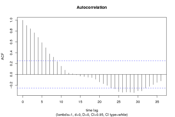
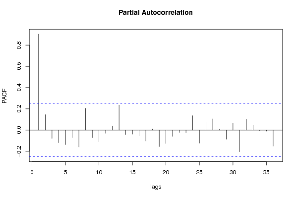
Title produced by software

(Partial) Autocorrelation Function

Date of computation

Tue, 22 Dec 2009 03:45:15 -0700

Cite this page as follows

Statistical Computations at FreeStatistics.org, Office for Research Development and Education, URL https://freestatistics.org/blog/index.php?v=date/2009/Dec/22/t12614787779fliorttuw7s4yw.htm/, Retrieved Sat, 04 May 2024 18:49:39 +0000

Statistical Computations at FreeStatistics.org, Office for Research Development and Education, URL https://freestatistics.org/blog/index.php?pk=70426, Retrieved Sat, 04 May 2024 18:49:39 +0000

QR Codes:

Paste this QR Code to cite your computation.

Original text written by user:

IsPrivate?

No (this computation is public)

User-defined keywords

paper, TRA, inflatie1

Estimated Impact

177

Family? (F = Feedback message, R = changed R code, M = changed R Module, P = changed Parameters, D = changed Data)

-       [(Partial) Autocorrelation Function] [] [2009-12-22 10:45:15] [30f5b608e5a1bbbae86b1702c0071566] [Current]
-   PD    [(Partial) Autocorrelation Function] [] [2009-12-23 11:39:04] [0750c128064677e728c9436fc3f45ae7] 
-   PD    [(Partial) Autocorrelation Function] [] [2009-12-23 11:43:23] [0750c128064677e728c9436fc3f45ae7] 
- RMPD    [Variance Reduction Matrix] [] [2009-12-23 11:46:22] [0750c128064677e728c9436fc3f45ae7] 
- RMPD    [Spectral Analysis] [] [2009-12-23 11:49:02] [0750c128064677e728c9436fc3f45ae7] 
- RMPD    [Spectral Analysis] [] [2009-12-23 11:50:52] [0750c128064677e728c9436fc3f45ae7] 
- RMPD    [Standard Deviation-Mean Plot] [] [2009-12-23 11:52:37] [0750c128064677e728c9436fc3f45ae7] 
- RMPD      [(Partial) Autocorrelation Function] [] [2009-12-23 11:57:09] [0750c128064677e728c9436fc3f45ae7] 
- RMPD      [(Partial) Autocorrelation Function] [] [2009-12-23 11:59:58] [0750c128064677e728c9436fc3f45ae7] 
- RM D      [Variance Reduction Matrix] [] [2009-12-23 12:01:40] [0750c128064677e728c9436fc3f45ae7] 
- RMPD      [Spectral Analysis] [] [2009-12-23 12:07:28] [0750c128064677e728c9436fc3f45ae7] 
- RMPD      [Spectral Analysis] [] [2009-12-23 12:08:52] [0750c128064677e728c9436fc3f45ae7] 
-    D      [Standard Deviation-Mean Plot] [] [2009-12-23 12:10:30] [0750c128064677e728c9436fc3f45ae7] 
- RMPD      [ARIMA Backward Selection] [] [2009-12-23 12:14:39] [0750c128064677e728c9436fc3f45ae7] 
- RMPD      [Univariate Explorative Data Analysis] [] [2009-12-23 12:18:50] [0750c128064677e728c9436fc3f45ae7] 
- RMPD      [ARIMA Backward Selection] [] [2009-12-23 12:24:26] [0750c128064677e728c9436fc3f45ae7] 
- RMPD      [Univariate Explorative Data Analysis] [] [2009-12-23 12:27:59] [0750c128064677e728c9436fc3f45ae7] 
- RMPD      [ARIMA Backward Selection] [] [2009-12-23 12:32:33] [0750c128064677e728c9436fc3f45ae7] 
- RMPD      [Univariate Explorative Data Analysis] [] [2009-12-23 12:34:54] [0750c128064677e728c9436fc3f45ae7] 
- RMPD      [ARIMA Forecasting] [] [2009-12-23 12:40:08] [0750c128064677e728c9436fc3f45ae7] 
- RMPD      [ARIMA Forecasting] [] [2009-12-23 12:43:23] [0750c128064677e728c9436fc3f45ae7] 
- RMPD      [ARIMA Forecasting] [] [2009-12-23 12:45:30] [0750c128064677e728c9436fc3f45ae7] 

Feedback Forum

Post a new message

Dataseries X:

Download CSV

Histogram

Boxplots

1,1
1,2
1,1
1,2
1,4
1,5
1,5
1,8
1,6
1,5
1,4
1,4
1,4
1,4
1,5
1,4
1,1
1,1
0,9
0,9
0,9
0,9
1,1
1,3
1
1,1
1,4
1,4
1,3
1,4
1
1,8
1,5
1,5
1,4
1,6
1,6
1,6
1,4
1,7
1,8
1,9
2,2
2,1
2,4
2,6
2,8
2,7
2,6
2,9
2,8
2,2
2,2
2,2
2
2
1,7
1,4
1,3
1,4
1,3

Summary of computational transaction
Raw Input	view raw input (R code)
Raw Output	view raw output of R engine
Computing time	1 seconds
R Server	'Gwilym Jenkins' @ 72.249.127.135

\begin{tabular}{lllllllll}
\hline
Summary of computational transaction \tabularnewline
Raw Input & view raw input (R code)  \tabularnewline
Raw Output & view raw output of R engine  \tabularnewline
Computing time & 1 seconds \tabularnewline
R Server & 'Gwilym Jenkins' @ 72.249.127.135 \tabularnewline
\hline
\end{tabular}
%Source: https://freestatistics.org/blog/index.php?pk=70426&T=0

[TABLE]
[ROW][C]Summary of computational transaction[/C][/ROW]
[ROW][C]Raw Input[/C][C]view raw input (R code) [/C][/ROW]
[ROW][C]Raw Output[/C][C]view raw output of R engine [/C][/ROW]
[ROW][C]Computing time[/C][C]1 seconds[/C][/ROW]
[ROW][C]R Server[/C][C]'Gwilym Jenkins' @ 72.249.127.135[/C][/ROW]
[/TABLE]
Source: https://freestatistics.org/blog/index.php?pk=70426&T=0

Globally Unique Identifier (entire table): ba.freestatistics.org/blog/index.php?pk=70426&T=0

As an alternative you can also use a QR Code:

The GUIDs for individual cells are displayed in the table below:

Summary of computational transaction
Raw Input	view raw input (R code)
Raw Output	view raw output of R engine
Computing time	1 seconds
R Server	'Gwilym Jenkins' @ 72.249.127.135

Autocorrelation Function
Time lag k	ACF(k)	T-STAT	P-value
1	0.903559	7.057	0
2	0.843185	6.5855	0
3	0.768485	6.0021	0
4	0.683886	5.3413	1e-06
5	0.587588	4.5892	1.1e-05
6	0.493235	3.8523	0.000142
7	0.380247	2.9698	0.002128
8	0.32078	2.5054	0.007459
9	0.237047	1.8514	0.034477
10	0.153294	1.1973	0.117918
11	0.081444	0.6361	0.263546
12	0.028249	0.2206	0.413058
13	0.014125	0.1103	0.456259
14	-0.006811	-0.0532	0.478874
15	-0.030813	-0.2407	0.405315
16	-0.039968	-0.3122	0.377993
17	-0.05233	-0.4087	0.342092
18	-0.059163	-0.4621	0.322834
19	-0.088378	-0.6903	0.246326
20	-0.138152	-1.079	0.142418
21	-0.171175	-1.3369	0.093107
22	-0.202976	-1.5853	0.059036
23	-0.247841	-1.9357	0.028771
24	-0.266537	-2.0817	0.020786
25	-0.318836	-2.4902	0.007754
26	-0.330119	-2.5783	0.006179
27	-0.324611	-2.5353	0.006907
28	-0.327779	-2.56	0.00648
29	-0.334693	-2.614	0.005628
30	-0.302395	-2.3618	0.010698
31	-0.304503	-2.3782	0.010271
32	-0.252328	-1.9707	0.026648
33	-0.22011	-1.7191	0.045332
34	-0.187252	-1.4625	0.074371
35	-0.147581	-1.1526	0.126777
36	-0.120353	-0.94	0.175466

\begin{tabular}{lllllllll}
\hline
Autocorrelation Function \tabularnewline
Time lag k & ACF(k) & T-STAT & P-value \tabularnewline
1 & 0.903559 & 7.057 & 0 \tabularnewline
2 & 0.843185 & 6.5855 & 0 \tabularnewline
3 & 0.768485 & 6.0021 & 0 \tabularnewline
4 & 0.683886 & 5.3413 & 1e-06 \tabularnewline
5 & 0.587588 & 4.5892 & 1.1e-05 \tabularnewline
6 & 0.493235 & 3.8523 & 0.000142 \tabularnewline
7 & 0.380247 & 2.9698 & 0.002128 \tabularnewline
8 & 0.32078 & 2.5054 & 0.007459 \tabularnewline
9 & 0.237047 & 1.8514 & 0.034477 \tabularnewline
10 & 0.153294 & 1.1973 & 0.117918 \tabularnewline
11 & 0.081444 & 0.6361 & 0.263546 \tabularnewline
12 & 0.028249 & 0.2206 & 0.413058 \tabularnewline
13 & 0.014125 & 0.1103 & 0.456259 \tabularnewline
14 & -0.006811 & -0.0532 & 0.478874 \tabularnewline
15 & -0.030813 & -0.2407 & 0.405315 \tabularnewline
16 & -0.039968 & -0.3122 & 0.377993 \tabularnewline
17 & -0.05233 & -0.4087 & 0.342092 \tabularnewline
18 & -0.059163 & -0.4621 & 0.322834 \tabularnewline
19 & -0.088378 & -0.6903 & 0.246326 \tabularnewline
20 & -0.138152 & -1.079 & 0.142418 \tabularnewline
21 & -0.171175 & -1.3369 & 0.093107 \tabularnewline
22 & -0.202976 & -1.5853 & 0.059036 \tabularnewline
23 & -0.247841 & -1.9357 & 0.028771 \tabularnewline
24 & -0.266537 & -2.0817 & 0.020786 \tabularnewline
25 & -0.318836 & -2.4902 & 0.007754 \tabularnewline
26 & -0.330119 & -2.5783 & 0.006179 \tabularnewline
27 & -0.324611 & -2.5353 & 0.006907 \tabularnewline
28 & -0.327779 & -2.56 & 0.00648 \tabularnewline
29 & -0.334693 & -2.614 & 0.005628 \tabularnewline
30 & -0.302395 & -2.3618 & 0.010698 \tabularnewline
31 & -0.304503 & -2.3782 & 0.010271 \tabularnewline
32 & -0.252328 & -1.9707 & 0.026648 \tabularnewline
33 & -0.22011 & -1.7191 & 0.045332 \tabularnewline
34 & -0.187252 & -1.4625 & 0.074371 \tabularnewline
35 & -0.147581 & -1.1526 & 0.126777 \tabularnewline
36 & -0.120353 & -0.94 & 0.175466 \tabularnewline
\hline
\end{tabular}
%Source: https://freestatistics.org/blog/index.php?pk=70426&T=1

[TABLE]
[ROW][C]Autocorrelation Function[/C][/ROW]
[ROW][C]Time lag k[/C][C]ACF(k)[/C][C]T-STAT[/C][C]P-value[/C][/ROW]
[ROW][C]1[/C][C]0.903559[/C][C]7.057[/C][C]0[/C][/ROW]
[ROW][C]2[/C][C]0.843185[/C][C]6.5855[/C][C]0[/C][/ROW]
[ROW][C]3[/C][C]0.768485[/C][C]6.0021[/C][C]0[/C][/ROW]
[ROW][C]4[/C][C]0.683886[/C][C]5.3413[/C][C]1e-06[/C][/ROW]
[ROW][C]5[/C][C]0.587588[/C][C]4.5892[/C][C]1.1e-05[/C][/ROW]
[ROW][C]6[/C][C]0.493235[/C][C]3.8523[/C][C]0.000142[/C][/ROW]
[ROW][C]7[/C][C]0.380247[/C][C]2.9698[/C][C]0.002128[/C][/ROW]
[ROW][C]8[/C][C]0.32078[/C][C]2.5054[/C][C]0.007459[/C][/ROW]
[ROW][C]9[/C][C]0.237047[/C][C]1.8514[/C][C]0.034477[/C][/ROW]
[ROW][C]10[/C][C]0.153294[/C][C]1.1973[/C][C]0.117918[/C][/ROW]
[ROW][C]11[/C][C]0.081444[/C][C]0.6361[/C][C]0.263546[/C][/ROW]
[ROW][C]12[/C][C]0.028249[/C][C]0.2206[/C][C]0.413058[/C][/ROW]
[ROW][C]13[/C][C]0.014125[/C][C]0.1103[/C][C]0.456259[/C][/ROW]
[ROW][C]14[/C][C]-0.006811[/C][C]-0.0532[/C][C]0.478874[/C][/ROW]
[ROW][C]15[/C][C]-0.030813[/C][C]-0.2407[/C][C]0.405315[/C][/ROW]
[ROW][C]16[/C][C]-0.039968[/C][C]-0.3122[/C][C]0.377993[/C][/ROW]
[ROW][C]17[/C][C]-0.05233[/C][C]-0.4087[/C][C]0.342092[/C][/ROW]
[ROW][C]18[/C][C]-0.059163[/C][C]-0.4621[/C][C]0.322834[/C][/ROW]
[ROW][C]19[/C][C]-0.088378[/C][C]-0.6903[/C][C]0.246326[/C][/ROW]
[ROW][C]20[/C][C]-0.138152[/C][C]-1.079[/C][C]0.142418[/C][/ROW]
[ROW][C]21[/C][C]-0.171175[/C][C]-1.3369[/C][C]0.093107[/C][/ROW]
[ROW][C]22[/C][C]-0.202976[/C][C]-1.5853[/C][C]0.059036[/C][/ROW]
[ROW][C]23[/C][C]-0.247841[/C][C]-1.9357[/C][C]0.028771[/C][/ROW]
[ROW][C]24[/C][C]-0.266537[/C][C]-2.0817[/C][C]0.020786[/C][/ROW]
[ROW][C]25[/C][C]-0.318836[/C][C]-2.4902[/C][C]0.007754[/C][/ROW]
[ROW][C]26[/C][C]-0.330119[/C][C]-2.5783[/C][C]0.006179[/C][/ROW]
[ROW][C]27[/C][C]-0.324611[/C][C]-2.5353[/C][C]0.006907[/C][/ROW]
[ROW][C]28[/C][C]-0.327779[/C][C]-2.56[/C][C]0.00648[/C][/ROW]
[ROW][C]29[/C][C]-0.334693[/C][C]-2.614[/C][C]0.005628[/C][/ROW]
[ROW][C]30[/C][C]-0.302395[/C][C]-2.3618[/C][C]0.010698[/C][/ROW]
[ROW][C]31[/C][C]-0.304503[/C][C]-2.3782[/C][C]0.010271[/C][/ROW]
[ROW][C]32[/C][C]-0.252328[/C][C]-1.9707[/C][C]0.026648[/C][/ROW]
[ROW][C]33[/C][C]-0.22011[/C][C]-1.7191[/C][C]0.045332[/C][/ROW]
[ROW][C]34[/C][C]-0.187252[/C][C]-1.4625[/C][C]0.074371[/C][/ROW]
[ROW][C]35[/C][C]-0.147581[/C][C]-1.1526[/C][C]0.126777[/C][/ROW]
[ROW][C]36[/C][C]-0.120353[/C][C]-0.94[/C][C]0.175466[/C][/ROW]
[/TABLE]
Source: https://freestatistics.org/blog/index.php?pk=70426&T=1

Globally Unique Identifier (entire table): ba.freestatistics.org/blog/index.php?pk=70426&T=1

As an alternative you can also use a QR Code:

The GUIDs for individual cells are displayed in the table below:

Autocorrelation Function
Time lag k	ACF(k)	T-STAT	P-value
1	0.903559	7.057	0
2	0.843185	6.5855	0
3	0.768485	6.0021	0
4	0.683886	5.3413	1e-06
5	0.587588	4.5892	1.1e-05
6	0.493235	3.8523	0.000142
7	0.380247	2.9698	0.002128
8	0.32078	2.5054	0.007459
9	0.237047	1.8514	0.034477
10	0.153294	1.1973	0.117918
11	0.081444	0.6361	0.263546
12	0.028249	0.2206	0.413058
13	0.014125	0.1103	0.456259
14	-0.006811	-0.0532	0.478874
15	-0.030813	-0.2407	0.405315
16	-0.039968	-0.3122	0.377993
17	-0.05233	-0.4087	0.342092
18	-0.059163	-0.4621	0.322834
19	-0.088378	-0.6903	0.246326
20	-0.138152	-1.079	0.142418
21	-0.171175	-1.3369	0.093107
22	-0.202976	-1.5853	0.059036
23	-0.247841	-1.9357	0.028771
24	-0.266537	-2.0817	0.020786
25	-0.318836	-2.4902	0.007754
26	-0.330119	-2.5783	0.006179
27	-0.324611	-2.5353	0.006907
28	-0.327779	-2.56	0.00648
29	-0.334693	-2.614	0.005628
30	-0.302395	-2.3618	0.010698
31	-0.304503	-2.3782	0.010271
32	-0.252328	-1.9707	0.026648
33	-0.22011	-1.7191	0.045332
34	-0.187252	-1.4625	0.074371
35	-0.147581	-1.1526	0.126777
36	-0.120353	-0.94	0.175466

Partial Autocorrelation Function
Time lag k	PACF(k)	T-STAT	P-value
1	0.903559	7.057	0
2	0.145801	1.1387	0.129632
3	-0.078151	-0.6104	0.27194
4	-0.118626	-0.9265	0.178918
5	-0.13716	-1.0713	0.144137
6	-0.070791	-0.5529	0.291177
7	-0.159818	-1.2482	0.10836
8	0.20465	1.5984	0.057564
9	-0.070989	-0.5544	0.290651
10	-0.110963	-0.8667	0.194765
11	-0.030482	-0.2381	0.406311
12	0.039873	0.3114	0.378272
13	0.235886	1.8423	0.035144
14	-0.041664	-0.3254	0.372995
15	-0.038329	-0.2994	0.382842
16	-0.055937	-0.4369	0.33187
17	-0.10351	-0.8084	0.210989
18	0.010794	0.0843	0.466545
19	-0.155416	-1.2138	0.114744
20	-0.125688	-0.9817	0.165074
21	-0.059073	-0.4614	0.323086
22	-0.02207	-0.1724	0.431859
23	-0.025669	-0.2005	0.420886
24	0.135589	1.059	0.146891
25	-0.122687	-0.9582	0.170869
26	0.07497	0.5855	0.280175
27	0.106936	0.8352	0.203434
28	0.007804	0.061	0.475798
29	-0.085745	-0.6697	0.252791
30	0.062897	0.4912	0.312509
31	-0.204172	-1.5946	0.057982
32	0.10181	0.7952	0.214801
33	0.045958	0.3589	0.360437
34	-0.008363	-0.0653	0.474068
35	-0.009797	-0.0765	0.469629
36	-0.150763	-1.1775	0.121786

\begin{tabular}{lllllllll}
\hline
Partial Autocorrelation Function \tabularnewline
Time lag k & PACF(k) & T-STAT & P-value \tabularnewline
1 & 0.903559 & 7.057 & 0 \tabularnewline
2 & 0.145801 & 1.1387 & 0.129632 \tabularnewline
3 & -0.078151 & -0.6104 & 0.27194 \tabularnewline
4 & -0.118626 & -0.9265 & 0.178918 \tabularnewline
5 & -0.13716 & -1.0713 & 0.144137 \tabularnewline
6 & -0.070791 & -0.5529 & 0.291177 \tabularnewline
7 & -0.159818 & -1.2482 & 0.10836 \tabularnewline
8 & 0.20465 & 1.5984 & 0.057564 \tabularnewline
9 & -0.070989 & -0.5544 & 0.290651 \tabularnewline
10 & -0.110963 & -0.8667 & 0.194765 \tabularnewline
11 & -0.030482 & -0.2381 & 0.406311 \tabularnewline
12 & 0.039873 & 0.3114 & 0.378272 \tabularnewline
13 & 0.235886 & 1.8423 & 0.035144 \tabularnewline
14 & -0.041664 & -0.3254 & 0.372995 \tabularnewline
15 & -0.038329 & -0.2994 & 0.382842 \tabularnewline
16 & -0.055937 & -0.4369 & 0.33187 \tabularnewline
17 & -0.10351 & -0.8084 & 0.210989 \tabularnewline
18 & 0.010794 & 0.0843 & 0.466545 \tabularnewline
19 & -0.155416 & -1.2138 & 0.114744 \tabularnewline
20 & -0.125688 & -0.9817 & 0.165074 \tabularnewline
21 & -0.059073 & -0.4614 & 0.323086 \tabularnewline
22 & -0.02207 & -0.1724 & 0.431859 \tabularnewline
23 & -0.025669 & -0.2005 & 0.420886 \tabularnewline
24 & 0.135589 & 1.059 & 0.146891 \tabularnewline
25 & -0.122687 & -0.9582 & 0.170869 \tabularnewline
26 & 0.07497 & 0.5855 & 0.280175 \tabularnewline
27 & 0.106936 & 0.8352 & 0.203434 \tabularnewline
28 & 0.007804 & 0.061 & 0.475798 \tabularnewline
29 & -0.085745 & -0.6697 & 0.252791 \tabularnewline
30 & 0.062897 & 0.4912 & 0.312509 \tabularnewline
31 & -0.204172 & -1.5946 & 0.057982 \tabularnewline
32 & 0.10181 & 0.7952 & 0.214801 \tabularnewline
33 & 0.045958 & 0.3589 & 0.360437 \tabularnewline
34 & -0.008363 & -0.0653 & 0.474068 \tabularnewline
35 & -0.009797 & -0.0765 & 0.469629 \tabularnewline
36 & -0.150763 & -1.1775 & 0.121786 \tabularnewline
\hline
\end{tabular}
%Source: https://freestatistics.org/blog/index.php?pk=70426&T=2

[TABLE]
[ROW][C]Partial Autocorrelation Function[/C][/ROW]
[ROW][C]Time lag k[/C][C]PACF(k)[/C][C]T-STAT[/C][C]P-value[/C][/ROW]
[ROW][C]1[/C][C]0.903559[/C][C]7.057[/C][C]0[/C][/ROW]
[ROW][C]2[/C][C]0.145801[/C][C]1.1387[/C][C]0.129632[/C][/ROW]
[ROW][C]3[/C][C]-0.078151[/C][C]-0.6104[/C][C]0.27194[/C][/ROW]
[ROW][C]4[/C][C]-0.118626[/C][C]-0.9265[/C][C]0.178918[/C][/ROW]
[ROW][C]5[/C][C]-0.13716[/C][C]-1.0713[/C][C]0.144137[/C][/ROW]
[ROW][C]6[/C][C]-0.070791[/C][C]-0.5529[/C][C]0.291177[/C][/ROW]
[ROW][C]7[/C][C]-0.159818[/C][C]-1.2482[/C][C]0.10836[/C][/ROW]
[ROW][C]8[/C][C]0.20465[/C][C]1.5984[/C][C]0.057564[/C][/ROW]
[ROW][C]9[/C][C]-0.070989[/C][C]-0.5544[/C][C]0.290651[/C][/ROW]
[ROW][C]10[/C][C]-0.110963[/C][C]-0.8667[/C][C]0.194765[/C][/ROW]
[ROW][C]11[/C][C]-0.030482[/C][C]-0.2381[/C][C]0.406311[/C][/ROW]
[ROW][C]12[/C][C]0.039873[/C][C]0.3114[/C][C]0.378272[/C][/ROW]
[ROW][C]13[/C][C]0.235886[/C][C]1.8423[/C][C]0.035144[/C][/ROW]
[ROW][C]14[/C][C]-0.041664[/C][C]-0.3254[/C][C]0.372995[/C][/ROW]
[ROW][C]15[/C][C]-0.038329[/C][C]-0.2994[/C][C]0.382842[/C][/ROW]
[ROW][C]16[/C][C]-0.055937[/C][C]-0.4369[/C][C]0.33187[/C][/ROW]
[ROW][C]17[/C][C]-0.10351[/C][C]-0.8084[/C][C]0.210989[/C][/ROW]
[ROW][C]18[/C][C]0.010794[/C][C]0.0843[/C][C]0.466545[/C][/ROW]
[ROW][C]19[/C][C]-0.155416[/C][C]-1.2138[/C][C]0.114744[/C][/ROW]
[ROW][C]20[/C][C]-0.125688[/C][C]-0.9817[/C][C]0.165074[/C][/ROW]
[ROW][C]21[/C][C]-0.059073[/C][C]-0.4614[/C][C]0.323086[/C][/ROW]
[ROW][C]22[/C][C]-0.02207[/C][C]-0.1724[/C][C]0.431859[/C][/ROW]
[ROW][C]23[/C][C]-0.025669[/C][C]-0.2005[/C][C]0.420886[/C][/ROW]
[ROW][C]24[/C][C]0.135589[/C][C]1.059[/C][C]0.146891[/C][/ROW]
[ROW][C]25[/C][C]-0.122687[/C][C]-0.9582[/C][C]0.170869[/C][/ROW]
[ROW][C]26[/C][C]0.07497[/C][C]0.5855[/C][C]0.280175[/C][/ROW]
[ROW][C]27[/C][C]0.106936[/C][C]0.8352[/C][C]0.203434[/C][/ROW]
[ROW][C]28[/C][C]0.007804[/C][C]0.061[/C][C]0.475798[/C][/ROW]
[ROW][C]29[/C][C]-0.085745[/C][C]-0.6697[/C][C]0.252791[/C][/ROW]
[ROW][C]30[/C][C]0.062897[/C][C]0.4912[/C][C]0.312509[/C][/ROW]
[ROW][C]31[/C][C]-0.204172[/C][C]-1.5946[/C][C]0.057982[/C][/ROW]
[ROW][C]32[/C][C]0.10181[/C][C]0.7952[/C][C]0.214801[/C][/ROW]
[ROW][C]33[/C][C]0.045958[/C][C]0.3589[/C][C]0.360437[/C][/ROW]
[ROW][C]34[/C][C]-0.008363[/C][C]-0.0653[/C][C]0.474068[/C][/ROW]
[ROW][C]35[/C][C]-0.009797[/C][C]-0.0765[/C][C]0.469629[/C][/ROW]
[ROW][C]36[/C][C]-0.150763[/C][C]-1.1775[/C][C]0.121786[/C][/ROW]
[/TABLE]
Source: https://freestatistics.org/blog/index.php?pk=70426&T=2

Globally Unique Identifier (entire table): ba.freestatistics.org/blog/index.php?pk=70426&T=2

As an alternative you can also use a QR Code:

The GUIDs for individual cells are displayed in the table below:

Partial Autocorrelation Function
Time lag k	PACF(k)	T-STAT	P-value
1	0.903559	7.057	0
2	0.145801	1.1387	0.129632
3	-0.078151	-0.6104	0.27194
4	-0.118626	-0.9265	0.178918
5	-0.13716	-1.0713	0.144137
6	-0.070791	-0.5529	0.291177
7	-0.159818	-1.2482	0.10836
8	0.20465	1.5984	0.057564
9	-0.070989	-0.5544	0.290651
10	-0.110963	-0.8667	0.194765
11	-0.030482	-0.2381	0.406311
12	0.039873	0.3114	0.378272
13	0.235886	1.8423	0.035144
14	-0.041664	-0.3254	0.372995
15	-0.038329	-0.2994	0.382842
16	-0.055937	-0.4369	0.33187
17	-0.10351	-0.8084	0.210989
18	0.010794	0.0843	0.466545
19	-0.155416	-1.2138	0.114744
20	-0.125688	-0.9817	0.165074
21	-0.059073	-0.4614	0.323086
22	-0.02207	-0.1724	0.431859
23	-0.025669	-0.2005	0.420886
24	0.135589	1.059	0.146891
25	-0.122687	-0.9582	0.170869
26	0.07497	0.5855	0.280175
27	0.106936	0.8352	0.203434
28	0.007804	0.061	0.475798
29	-0.085745	-0.6697	0.252791
30	0.062897	0.4912	0.312509
31	-0.204172	-1.5946	0.057982
32	0.10181	0.7952	0.214801
33	0.045958	0.3589	0.360437
34	-0.008363	-0.0653	0.474068
35	-0.009797	-0.0765	0.469629
36	-0.150763	-1.1775	0.121786

Figure 1

PNG link

Postscript link

PDF link

Figure 2

PNG link

Postscript link

PDF link

Parameters (Session):

par1 = 36 ; par2 = 1 ; par3 = 0 ; par4 = 0 ; par5 = 12 ; par6 = White Noise ; par7 = 0.95 ;

Parameters (R input):

par1 = 36 ; par2 = 1 ; par3 = 0 ; par4 = 0 ; par5 = 12 ; par6 = White Noise ; par7 = 0.95 ;

R code (references can be found in the software module):

if (par1 == 'Default') {
par1 = 10*log10(length(x))
} else {
par1 <- as.numeric(par1)
}
par2 <- as.numeric(par2)
par3 <- as.numeric(par3)
par4 <- as.numeric(par4)
par5 <- as.numeric(par5)
if (par6 == 'White Noise') par6 <- 'white' else par6 <- 'ma'
par7 <- as.numeric(par7)
if (par2 == 0) {
x <- log(x)
} else {
x <- (x ^ par2 - 1) / par2
}
if (par3 > 0) x <- diff(x,lag=1,difference=par3)
if (par4 > 0) x <- diff(x,lag=par5,difference=par4)
bitmap(file='pic1.png')
racf <- acf(x, par1, main='Autocorrelation', xlab='time lag', ylab='ACF', ci.type=par6, ci=par7, sub=paste('(lambda=',par2,', d=',par3,', D=',par4,', CI=', par7, ', CI type=',par6,')',sep=''))
dev.off()
bitmap(file='pic2.png')
rpacf <- pacf(x,par1,main='Partial Autocorrelation',xlab='lags',ylab='PACF')
dev.off()
(myacf <- c(racf$acf))
(mypacf <- c(rpacf$acf))
lengthx <- length(x)
sqrtn <- sqrt(lengthx)
load(file='createtable')
a<-table.start()
a<-table.row.start(a)
a<-table.element(a,'Autocorrelation Function',4,TRUE)
a<-table.row.end(a)
a<-table.row.start(a)
a<-table.element(a,'Time lag k',header=TRUE)
a<-table.element(a,hyperlink('basics.htm','ACF(k)','click here for more information about the Autocorrelation Function'),header=TRUE)
a<-table.element(a,'T-STAT',header=TRUE)
a<-table.element(a,'P-value',header=TRUE)
a<-table.row.end(a)
for (i in 2:(par1+1)) {
a<-table.row.start(a)
a<-table.element(a,i-1,header=TRUE)
a<-table.element(a,round(myacf[i],6))
mytstat <- myacf[i]*sqrtn
a<-table.element(a,round(mytstat,4))
a<-table.element(a,round(1-pt(abs(mytstat),lengthx),6))
a<-table.row.end(a)
}
a<-table.end(a)
table.save(a,file='mytable.tab')
a<-table.start()
a<-table.row.start(a)
a<-table.element(a,'Partial Autocorrelation Function',4,TRUE)
a<-table.row.end(a)
a<-table.row.start(a)
a<-table.element(a,'Time lag k',header=TRUE)
a<-table.element(a,hyperlink('basics.htm','PACF(k)','click here for more information about the Partial Autocorrelation Function'),header=TRUE)
a<-table.element(a,'T-STAT',header=TRUE)
a<-table.element(a,'P-value',header=TRUE)
a<-table.row.end(a)
for (i in 1:par1) {
a<-table.row.start(a)
a<-table.element(a,i,header=TRUE)
a<-table.element(a,round(mypacf[i],6))
mytstat <- mypacf[i]*sqrtn
a<-table.element(a,round(mytstat,4))
a<-table.element(a,round(1-pt(abs(mytstat),lengthx),6))
a<-table.row.end(a)
}
a<-table.end(a)
table.save(a,file='mytable1.tab')

Free Statistics

Description of Statistical Computation

Tree of Dependent Computations

Dataset

Tables (Output of Computation)

Figures (Output of Computation)

Input Parameters & R Code