Free Statistics
of Irreproducible Research!
Description of Statistical Computation | |||||||||||||||||||||||||||||||||||||||||||||||||||||
|---|---|---|---|---|---|---|---|---|---|---|---|---|---|---|---|---|---|---|---|---|---|---|---|---|---|---|---|---|---|---|---|---|---|---|---|---|---|---|---|---|---|---|---|---|---|---|---|---|---|---|---|---|---|
| Author's title | |||||||||||||||||||||||||||||||||||||||||||||||||||||
| Author | *The author of this computation has been verified* | ||||||||||||||||||||||||||||||||||||||||||||||||||||
| R Software Module | rwasp_edauni.wasp | ||||||||||||||||||||||||||||||||||||||||||||||||||||
| Title produced by software | Univariate Explorative Data Analysis | ||||||||||||||||||||||||||||||||||||||||||||||||||||
| Date of computation | Mon, 28 Dec 2009 07:10:03 -0700 | ||||||||||||||||||||||||||||||||||||||||||||||||||||
| Cite this page as follows | Statistical Computations at FreeStatistics.org, Office for Research Development and Education, URL https://freestatistics.org/blog/index.php?v=date/2009/Dec/28/t1262009449c9y7bdjuxnx169q.htm/, Retrieved Sun, 05 May 2024 00:00:20 +0000 | ||||||||||||||||||||||||||||||||||||||||||||||||||||
| Statistical Computations at FreeStatistics.org, Office for Research Development and Education, URL https://freestatistics.org/blog/index.php?pk=70972, Retrieved Sun, 05 May 2024 00:00:20 +0000 | |||||||||||||||||||||||||||||||||||||||||||||||||||||
| QR Codes: | |||||||||||||||||||||||||||||||||||||||||||||||||||||
|
| |||||||||||||||||||||||||||||||||||||||||||||||||||||
| Original text written by user: | |||||||||||||||||||||||||||||||||||||||||||||||||||||
| IsPrivate? | No (this computation is public) | ||||||||||||||||||||||||||||||||||||||||||||||||||||
| User-defined keywords | Paper | ||||||||||||||||||||||||||||||||||||||||||||||||||||
| Estimated Impact | 133 | ||||||||||||||||||||||||||||||||||||||||||||||||||||
Tree of Dependent Computations | |||||||||||||||||||||||||||||||||||||||||||||||||||||
| Family? (F = Feedback message, R = changed R code, M = changed R Module, P = changed Parameters, D = changed Data) | |||||||||||||||||||||||||||||||||||||||||||||||||||||
| - [Bivariate Data Series] [Bivariate dataset] [2008-01-05 23:51:08] [74be16979710d4c4e7c6647856088456] - RMPD [Univariate Explorative Data Analysis] [SHW_WS4_Q3] [2009-10-23 09:32:44] [8b1aef4e7013bd33fbc2a5833375c5f5] - RM D [Univariate Explorative Data Analysis] [Assumpties_1&2] [2009-12-28 14:10:03] [5b5bced41faf164488f2c271c918b21f] [Current] | |||||||||||||||||||||||||||||||||||||||||||||||||||||
| Feedback Forum | |||||||||||||||||||||||||||||||||||||||||||||||||||||
Post a new message | |||||||||||||||||||||||||||||||||||||||||||||||||||||
Dataset | |||||||||||||||||||||||||||||||||||||||||||||||||||||
| Dataseries X: | |||||||||||||||||||||||||||||||||||||||||||||||||||||
-564,5024598 -563,2868321 -562,6092123 -561,7289219 -561,1287748 -560,5596749 -559,6534424 -559,3645562 -559,116752 -558,4967141 -558,503492 -558,5209538 -557,0677242 -555,4223769 -555,097832 -553,4948419 -552,6864705 -551,9045613 -551,1060444 -550,6091745 -550,3793745 -550,1054427 -549,8546061 -548,844823 -548,5840858 -548,617565 -548,2909357 -548,0708184 -548,0966998 -547,8101955 -547,5950275 -547,5658663 -547,3702787 -547,351529 -547,0982745 -547,1077645 -546,8794054 -546,6257451 -546,3368134 -545,3938705 -544,2206706 -543,9774587 -543,7544865 -543,5103391 -543,3197988 -543,0791292 -543,0649124 -542,8425928 -542,6238584 -542,4033326 -542,1077162 -541,937633 -541,6831711 -541,6820682 -541,4839707 -541,4566051 -540,3987325 -540,1404426 -536,6900434 -535,8951806 | |||||||||||||||||||||||||||||||||||||||||||||||||||||
Tables (Output of Computation) | |||||||||||||||||||||||||||||||||||||||||||||||||||||
| |||||||||||||||||||||||||||||||||||||||||||||||||||||
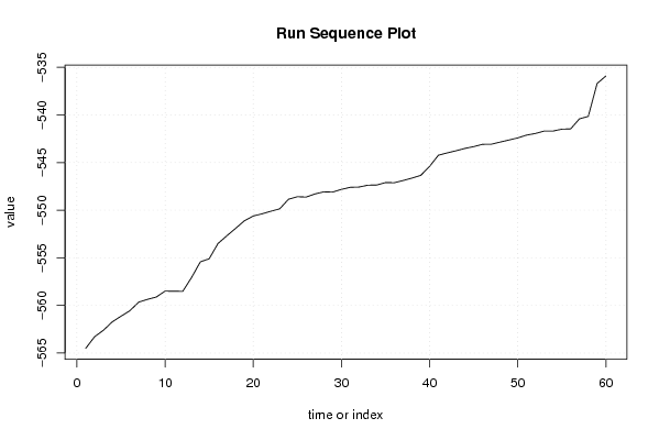
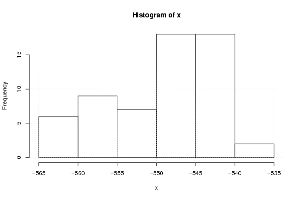
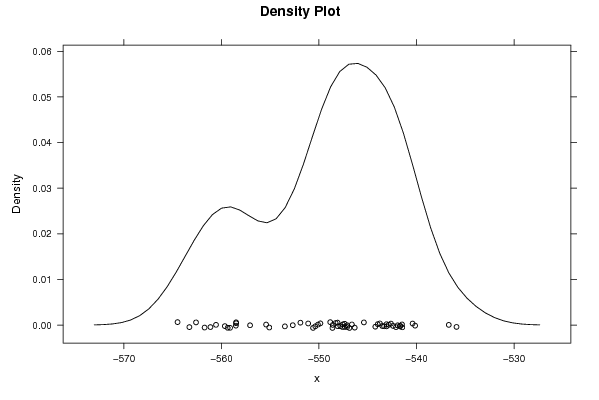
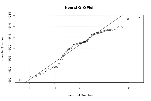
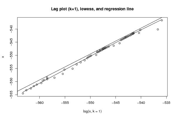
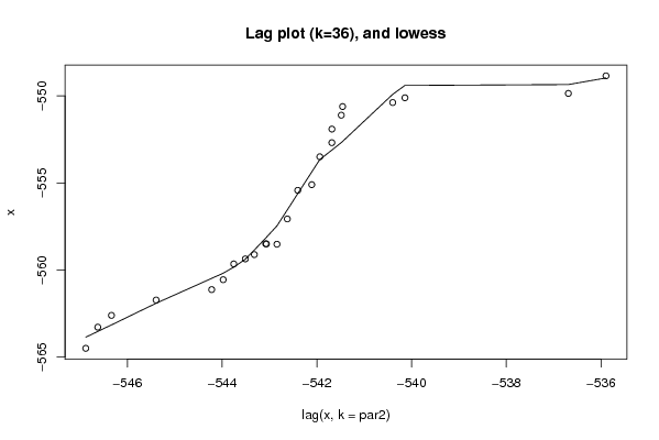
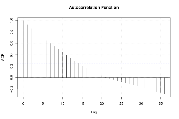
Figures (Output of Computation) | |||||||||||||||||||||||||||||||||||||||||||||||||||||
Input Parameters & R Code | |||||||||||||||||||||||||||||||||||||||||||||||||||||
| Parameters (Session): | |||||||||||||||||||||||||||||||||||||||||||||||||||||
| par1 = 0 ; par2 = 36 ; | |||||||||||||||||||||||||||||||||||||||||||||||||||||
| Parameters (R input): | |||||||||||||||||||||||||||||||||||||||||||||||||||||
| par1 = 0 ; par2 = 36 ; | |||||||||||||||||||||||||||||||||||||||||||||||||||||
| R code (references can be found in the software module): | |||||||||||||||||||||||||||||||||||||||||||||||||||||
par1 <- as.numeric(par1) | |||||||||||||||||||||||||||||||||||||||||||||||||||||