Free Statistics
of Irreproducible Research!
Description of Statistical Computation | |||||||||||||||||||||
|---|---|---|---|---|---|---|---|---|---|---|---|---|---|---|---|---|---|---|---|---|---|
| Author's title | |||||||||||||||||||||
| Author | *The author of this computation has been verified* | ||||||||||||||||||||
| R Software Module | rwasp_cloud.wasp | ||||||||||||||||||||
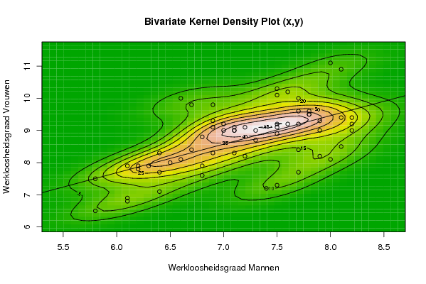
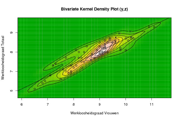
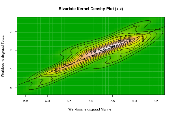
| Title produced by software | Trivariate Scatterplots | ||||||||||||||||||||
| Date of computation | Tue, 03 Nov 2009 10:42:05 -0700 | ||||||||||||||||||||
| Cite this page as follows | Statistical Computations at FreeStatistics.org, Office for Research Development and Education, URL https://freestatistics.org/blog/index.php?v=date/2009/Nov/03/t1257270446i5cp3m1nv85dd1a.htm/, Retrieved Mon, 07 Jul 2025 05:23:03 +0000 | ||||||||||||||||||||
| Statistical Computations at FreeStatistics.org, Office for Research Development and Education, URL https://freestatistics.org/blog/index.php?pk=53269, Retrieved Mon, 07 Jul 2025 05:23:03 +0000 | |||||||||||||||||||||
| QR Codes: | |||||||||||||||||||||
|
| |||||||||||||||||||||
| Original text written by user: | |||||||||||||||||||||
| IsPrivate? | No (this computation is public) | ||||||||||||||||||||
| User-defined keywords | DSHW, SDHW | ||||||||||||||||||||
| Estimated Impact | 220 | ||||||||||||||||||||
Tree of Dependent Computations | |||||||||||||||||||||
| Family? (F = Feedback message, R = changed R code, M = changed R Module, P = changed Parameters, D = changed Data) | |||||||||||||||||||||
| - [Trivariate Scatterplots] [WS 5 1] [2009-10-28 22:35:45] [6e4e01d7eb22a9f33d58ebb35753a195] - MPD [Trivariate Scatterplots] [DSHW-WS5-Trivaria...] [2009-11-03 17:42:05] [36295456a56d4c7dcc9b9537ce63463b] [Current] - RMPD [Bivariate Explorative Data Analysis] [DSHW-WS5-Bivariat...] [2009-11-03 18:01:01] [f15cfb7053d35072d573abca87df96a0] - RMPD [Kendall tau Correlation Matrix] [Kendell Tau corre...] [2009-11-07 15:38:04] [d31db4f83c6a129f6d3e47077769e868] | |||||||||||||||||||||
| Feedback Forum | |||||||||||||||||||||
Post a new message | |||||||||||||||||||||
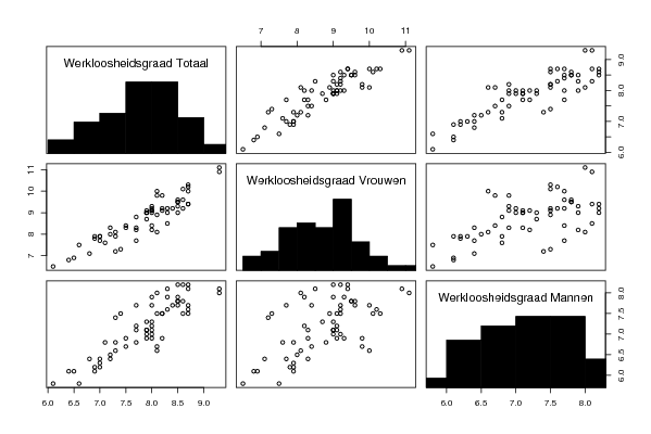
Dataset | |||||||||||||||||||||
| Dataseries X: | |||||||||||||||||||||
8 8,1 7,7 7,5 7,6 7,8 7,8 7,8 7,5 7,5 7,1 7,5 7,5 7,6 7,7 7,7 7,9 8,1 8,2 8,2 8,2 7,9 7,3 6,9 6,6 6,7 6,9 7 7,1 7,2 7,1 6,9 7 6,8 6,4 6,7 6,6 6,4 6,3 6,2 6,5 6,8 6,8 6,4 6,1 5,8 6,1 7,2 7,3 6,9 6,1 5,8 6,2 7,1 7,7 7,9 7,7 7,4 7,5 8 8,1 | |||||||||||||||||||||
| Dataseries Y: | |||||||||||||||||||||
11,1 10,9 10 9,2 9,2 9,5 9,6 9,5 9,1 8,9 9 10,1 10,3 10,2 9,6 9,2 9,3 9,4 9,4 9,2 9 9 9 9,8 10 9,8 9,3 9 9 9,1 9,1 9,1 9,2 8,8 8,3 8,4 8,1 7,7 7,9 7,9 8 7,9 7,6 7,1 6,8 6,5 6,9 8,2 8,7 8,3 7,9 7,5 7,8 8,3 8,4 8,2 7,7 7,2 7,3 8,1 8,5 | |||||||||||||||||||||
| Dataseries Z: | |||||||||||||||||||||
9,3 9,3 8,7 8,2 8,3 8,5 8,6 8,5 8,2 8,1 7,9 8,6 8,7 8,7 8,5 8,4 8,5 8,7 8,7 8,6 8,5 8,3 8 8,2 8,1 8,1 8 7,9 7,9 8 8 7,9 8 7,7 7,2 7,5 7,3 7 7 7 7,2 7,3 7,1 6,8 6,4 6,1 6,5 7,7 7,9 7,5 6,9 6,6 6,9 7,7 8 8 7,7 7,3 7,4 8,1 8,3 | |||||||||||||||||||||
Tables (Output of Computation) | |||||||||||||||||||||
| |||||||||||||||||||||
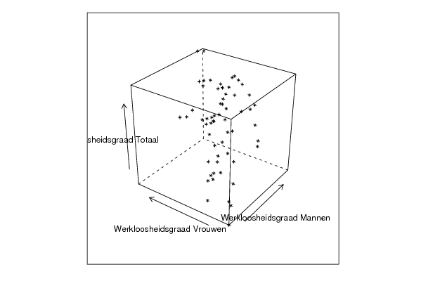
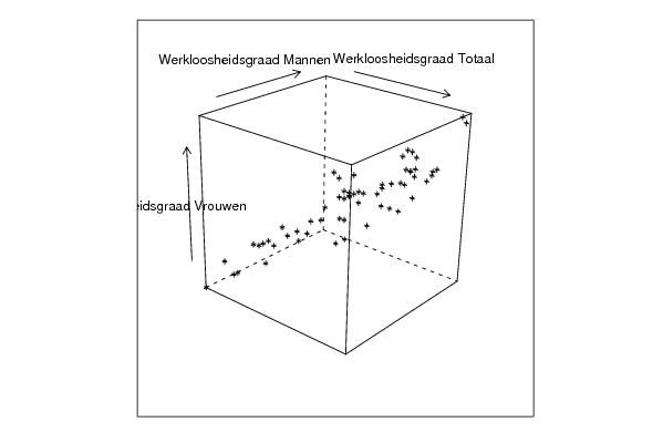
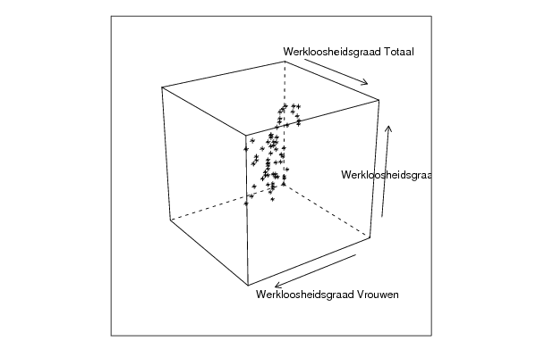
Figures (Output of Computation) | |||||||||||||||||||||
Input Parameters & R Code | |||||||||||||||||||||
| Parameters (Session): | |||||||||||||||||||||
| par1 = 50 ; par2 = 50 ; par3 = Y ; par4 = Y ; par5 = Werkloosheidsgraad Mannen ; par6 = Werkloosheidsgraad Vrouwen ; par7 = Werkloosheidsgraad Totaal ; | |||||||||||||||||||||
| Parameters (R input): | |||||||||||||||||||||
| par1 = 50 ; par2 = 50 ; par3 = Y ; par4 = Y ; par5 = Werkloosheidsgraad Mannen ; par6 = Werkloosheidsgraad Vrouwen ; par7 = Werkloosheidsgraad Totaal ; | |||||||||||||||||||||
| R code (references can be found in the software module): | |||||||||||||||||||||
x <- array(x,dim=c(length(x),1)) | |||||||||||||||||||||