Free Statistics
of Irreproducible Research!
Description of Statistical Computation | |||||||||||||||||||||||||||||||||||||||||||||||||||||||||||||||||
|---|---|---|---|---|---|---|---|---|---|---|---|---|---|---|---|---|---|---|---|---|---|---|---|---|---|---|---|---|---|---|---|---|---|---|---|---|---|---|---|---|---|---|---|---|---|---|---|---|---|---|---|---|---|---|---|---|---|---|---|---|---|---|---|---|---|
| Author's title | |||||||||||||||||||||||||||||||||||||||||||||||||||||||||||||||||
| Author | *The author of this computation has been verified* | ||||||||||||||||||||||||||||||||||||||||||||||||||||||||||||||||
| R Software Module | rwasp_edabi.wasp | ||||||||||||||||||||||||||||||||||||||||||||||||||||||||||||||||
| Title produced by software | Bivariate Explorative Data Analysis | ||||||||||||||||||||||||||||||||||||||||||||||||||||||||||||||||
| Date of computation | Tue, 03 Nov 2009 11:33:00 -0700 | ||||||||||||||||||||||||||||||||||||||||||||||||||||||||||||||||
| Cite this page as follows | Statistical Computations at FreeStatistics.org, Office for Research Development and Education, URL https://freestatistics.org/blog/index.php?v=date/2009/Nov/03/t1257273257gobe752f93qazz2.htm/, Retrieved Wed, 01 May 2024 16:37:12 +0000 | ||||||||||||||||||||||||||||||||||||||||||||||||||||||||||||||||
| Statistical Computations at FreeStatistics.org, Office for Research Development and Education, URL https://freestatistics.org/blog/index.php?pk=53315, Retrieved Wed, 01 May 2024 16:37:12 +0000 | |||||||||||||||||||||||||||||||||||||||||||||||||||||||||||||||||
| QR Codes: | |||||||||||||||||||||||||||||||||||||||||||||||||||||||||||||||||
|
| |||||||||||||||||||||||||||||||||||||||||||||||||||||||||||||||||
| Original text written by user: | |||||||||||||||||||||||||||||||||||||||||||||||||||||||||||||||||
| IsPrivate? | No (this computation is public) | ||||||||||||||||||||||||||||||||||||||||||||||||||||||||||||||||
| User-defined keywords | shwws5v1 | ||||||||||||||||||||||||||||||||||||||||||||||||||||||||||||||||
| Estimated Impact | 107 | ||||||||||||||||||||||||||||||||||||||||||||||||||||||||||||||||
Tree of Dependent Computations | |||||||||||||||||||||||||||||||||||||||||||||||||||||||||||||||||
| Family? (F = Feedback message, R = changed R code, M = changed R Module, P = changed Parameters, D = changed Data) | |||||||||||||||||||||||||||||||||||||||||||||||||||||||||||||||||
| - [Bivariate Data Series] [Bivariate dataset] [2008-01-05 23:51:08] [74be16979710d4c4e7c6647856088456] - RMPD [Bivariate Explorative Data Analysis] [] [2009-10-28 15:16:32] [5482608004c1d7bbf873930172393a2d] - D [Bivariate Explorative Data Analysis] [] [2009-10-28 16:44:36] [5482608004c1d7bbf873930172393a2d] - RMPD [Trivariate Scatterplots] [] [2009-11-03 17:57:36] [5482608004c1d7bbf873930172393a2d] - RMPD [Bivariate Explorative Data Analysis] [] [2009-11-03 18:33:00] [efdfe680cd785c4af09f858b30f777ec] [Current] - D [Bivariate Explorative Data Analysis] [workshop 5 bivari...] [2009-11-04 11:34:19] [af8eb90b4bf1bcfcc4325c143dbee260] - D [Bivariate Explorative Data Analysis] [Workshop 5 Bivari...] [2009-11-04 11:34:29] [b6394cb5c2dcec6d17418d3cdf42d699] - D [Bivariate Explorative Data Analysis] [Workshop 5, Bivar...] [2009-11-04 11:44:07] [aba88da643e3763d32ff92bd8f92a385] | |||||||||||||||||||||||||||||||||||||||||||||||||||||||||||||||||
| Feedback Forum | |||||||||||||||||||||||||||||||||||||||||||||||||||||||||||||||||
Post a new message | |||||||||||||||||||||||||||||||||||||||||||||||||||||||||||||||||
Dataset | |||||||||||||||||||||||||||||||||||||||||||||||||||||||||||||||||
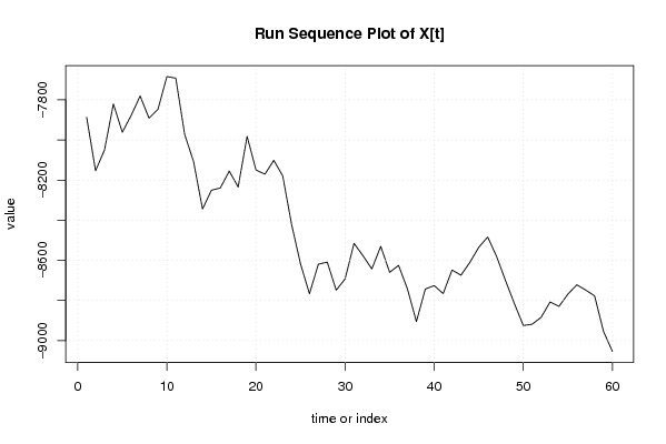
| Dataseries X: | |||||||||||||||||||||||||||||||||||||||||||||||||||||||||||||||||
-7887,38628 -8153,249971 -8050,245702 -7820,43309 -7961,598309 -7877,474807 -7781,108569 -7891,555768 -7847,376918 -7683,962074 -7692,226978 -7972,697994 -8108,607671 -8343,945823 -8250,612764 -8239,157028 -8155,088873 -8234,545434 -7982,266075 -8149,727729 -8170,722635 -8101,449194 -8179,134035 -8421,929572 -8617,979002 -8766,284799 -8618,868306 -8608,777983 -8748,581233 -8692,242257 -8515,081307 -8576,701438 -8642,645266 -8530,422903 -8659,69717 -8624,979149 -8743,290039 -8905,048128 -8742,865833 -8725,697994 -8765,611115 -8648,052397 -8673,760231 -8610,19215 -8534,813106 -8483,389724 -8580,503864 -8700,645266 -8816,079659 -8924,674177 -8917,935636 -8883,476455 -8807,16639 -8829,066705 -8768,618682 -8721,75499 -8748,015626 -8776,99855 -8954,624599 -9053,98065 | |||||||||||||||||||||||||||||||||||||||||||||||||||||||||||||||||
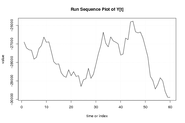
| Dataseries Y: | |||||||||||||||||||||||||||||||||||||||||||||||||||||||||||||||||
-26899,91791 -27221,72575 -27317,12474 -27344,50896 -27823,97196 -27724,58281 -27255,01638 -27091,98191 -26630,7997 -26910,7898 -26887,88832 -27413,60748 -27971,09017 -28096,30197 -28082,60737 -28558,43982 -28738,84374 -28804,92749 -28397,19356 -28720,79451 -28500,2773 -28755,97677 -28718,6024 -29299,81415 -28936,17381 -28881,42998 -28321,58768 -28861,07037 -28646,56793 -28114,43993 -27536,57794 -27082,29229 -26368,58303 -26969,47456 -27154,69128 -26624,19383 -26836,9672 -26906,70611 -26991,83909 -27604,60748 -27551,77498 -26686,30711 -26767,77016 -25811,18409 -25771,81463 -26344,60272 -26401,87366 -26360,58303 -26672,74555 -27176,85386 -27699,26757 -28752,41521 -28974,55803 -29436,92251 -29195,04078 -28833,23294 -28995,73045 -29580,32643 -29882,47418 -29891,00621 | |||||||||||||||||||||||||||||||||||||||||||||||||||||||||||||||||
Tables (Output of Computation) | |||||||||||||||||||||||||||||||||||||||||||||||||||||||||||||||||
| |||||||||||||||||||||||||||||||||||||||||||||||||||||||||||||||||
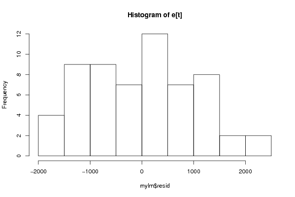
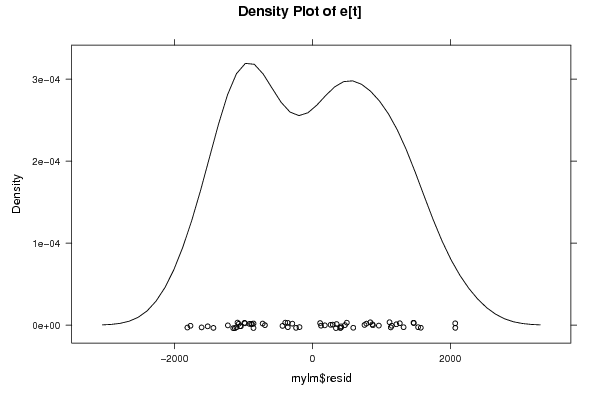
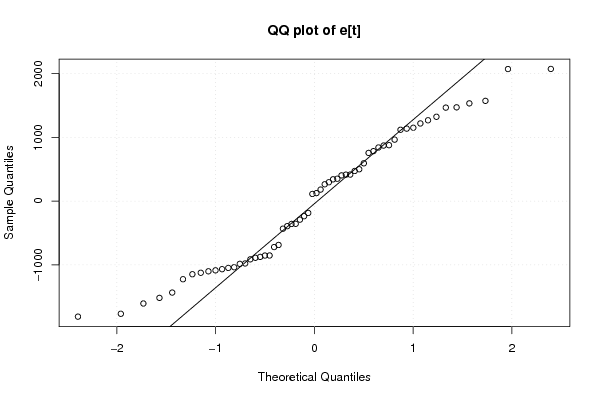
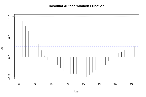
Figures (Output of Computation) | |||||||||||||||||||||||||||||||||||||||||||||||||||||||||||||||||
Input Parameters & R Code | |||||||||||||||||||||||||||||||||||||||||||||||||||||||||||||||||
| Parameters (Session): | |||||||||||||||||||||||||||||||||||||||||||||||||||||||||||||||||
| par1 = 0 ; par2 = 36 ; | |||||||||||||||||||||||||||||||||||||||||||||||||||||||||||||||||
| Parameters (R input): | |||||||||||||||||||||||||||||||||||||||||||||||||||||||||||||||||
| par1 = 0 ; par2 = 36 ; | |||||||||||||||||||||||||||||||||||||||||||||||||||||||||||||||||
| R code (references can be found in the software module): | |||||||||||||||||||||||||||||||||||||||||||||||||||||||||||||||||
par1 <- as.numeric(par1) | |||||||||||||||||||||||||||||||||||||||||||||||||||||||||||||||||