Free Statistics
of Irreproducible Research!
Description of Statistical Computation | |||||||||||||||||||||||||||||||||||||||||||||||||||||||||||||||||||||
|---|---|---|---|---|---|---|---|---|---|---|---|---|---|---|---|---|---|---|---|---|---|---|---|---|---|---|---|---|---|---|---|---|---|---|---|---|---|---|---|---|---|---|---|---|---|---|---|---|---|---|---|---|---|---|---|---|---|---|---|---|---|---|---|---|---|---|---|---|---|
| Author's title | |||||||||||||||||||||||||||||||||||||||||||||||||||||||||||||||||||||
| Author | *The author of this computation has been verified* | ||||||||||||||||||||||||||||||||||||||||||||||||||||||||||||||||||||
| R Software Module | rwasp_edabi.wasp | ||||||||||||||||||||||||||||||||||||||||||||||||||||||||||||||||||||
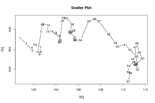
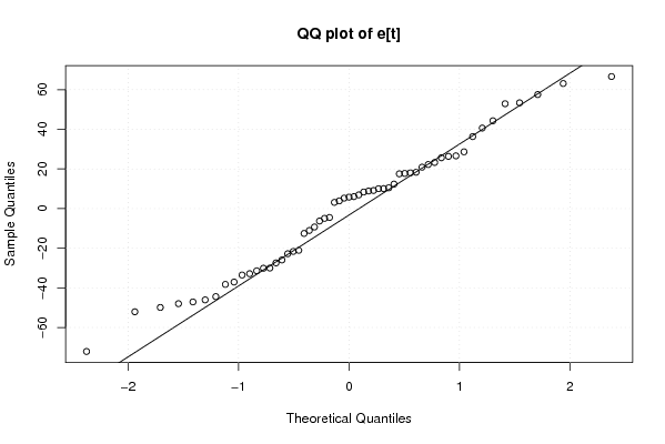
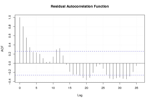
| Title produced by software | Bivariate Explorative Data Analysis | ||||||||||||||||||||||||||||||||||||||||||||||||||||||||||||||||||||
| Date of computation | Tue, 03 Nov 2009 12:54:11 -0700 | ||||||||||||||||||||||||||||||||||||||||||||||||||||||||||||||||||||
| Cite this page as follows | Statistical Computations at FreeStatistics.org, Office for Research Development and Education, URL https://freestatistics.org/blog/index.php?v=date/2009/Nov/03/t1257278109b3zjvyo1dpa4duk.htm/, Retrieved Wed, 01 May 2024 22:57:03 +0000 | ||||||||||||||||||||||||||||||||||||||||||||||||||||||||||||||||||||
| Statistical Computations at FreeStatistics.org, Office for Research Development and Education, URL https://freestatistics.org/blog/index.php?pk=53373, Retrieved Wed, 01 May 2024 22:57:03 +0000 | |||||||||||||||||||||||||||||||||||||||||||||||||||||||||||||||||||||
| QR Codes: | |||||||||||||||||||||||||||||||||||||||||||||||||||||||||||||||||||||
|
| |||||||||||||||||||||||||||||||||||||||||||||||||||||||||||||||||||||
| Original text written by user: | |||||||||||||||||||||||||||||||||||||||||||||||||||||||||||||||||||||
| IsPrivate? | No (this computation is public) | ||||||||||||||||||||||||||||||||||||||||||||||||||||||||||||||||||||
| User-defined keywords | |||||||||||||||||||||||||||||||||||||||||||||||||||||||||||||||||||||
| Estimated Impact | 162 | ||||||||||||||||||||||||||||||||||||||||||||||||||||||||||||||||||||
Tree of Dependent Computations | |||||||||||||||||||||||||||||||||||||||||||||||||||||||||||||||||||||
| Family? (F = Feedback message, R = changed R code, M = changed R Module, P = changed Parameters, D = changed Data) | |||||||||||||||||||||||||||||||||||||||||||||||||||||||||||||||||||||
| - [Trivariate Scatterplots] [] [2009-11-03 19:22:33] [134dc66689e3d457a82860db6471d419] - RMPD [Bivariate Explorative Data Analysis] [x en z] [2009-11-03 19:54:11] [4f297b039e1043ebee7ff7a83b1eaaaa] [Current] - D [Bivariate Explorative Data Analysis] [X en Z] [2009-11-05 10:36:43] [3425351e86519d261a643e224a0c8ee1] - D [Bivariate Explorative Data Analysis] [X en Z] [2009-11-05 10:36:43] [3425351e86519d261a643e224a0c8ee1] - D [Bivariate Explorative Data Analysis] [X en Z] [2009-11-05 10:36:43] [3425351e86519d261a643e224a0c8ee1] - D [Bivariate Explorative Data Analysis] [X en Z] [2009-11-05 10:36:43] [3425351e86519d261a643e224a0c8ee1] | |||||||||||||||||||||||||||||||||||||||||||||||||||||||||||||||||||||
| Feedback Forum | |||||||||||||||||||||||||||||||||||||||||||||||||||||||||||||||||||||
Post a new message | |||||||||||||||||||||||||||||||||||||||||||||||||||||||||||||||||||||
Dataset | |||||||||||||||||||||||||||||||||||||||||||||||||||||||||||||||||||||
| Dataseries X: | |||||||||||||||||||||||||||||||||||||||||||||||||||||||||||||||||||||
100.80 101.33 101.88 101.85 102.04 102.22 102.63 102.65 102.54 102.37 102.68 102.76 102.82 103.31 103.23 103.60 103.95 103.93 104.25 104.38 104.36 104.32 104.58 104.68 104.92 105.46 105.23 105.58 105.34 105.28 105.70 105.67 105.71 106.19 106.93 107.44 107.85 108.71 109.32 109.49 110.20 110.62 111.22 110.88 111.15 111.29 111.09 111.24 111.45 111.75 111.07 111.17 110.96 110.50 110.48 110.66 110.46 | |||||||||||||||||||||||||||||||||||||||||||||||||||||||||||||||||||||
| Dataseries Y: | |||||||||||||||||||||||||||||||||||||||||||||||||||||||||||||||||||||
578 565 547 555 562 561 555 544 537 543 594 611 613 611 594 595 591 589 584 573 567 569 621 629 628 612 595 597 593 590 580 574 573 573 620 626 620 588 566 557 561 549 532 526 511 499 555 565 542 527 510 514 517 508 493 490 469 | |||||||||||||||||||||||||||||||||||||||||||||||||||||||||||||||||||||
Tables (Output of Computation) | |||||||||||||||||||||||||||||||||||||||||||||||||||||||||||||||||||||
| |||||||||||||||||||||||||||||||||||||||||||||||||||||||||||||||||||||
Figures (Output of Computation) | |||||||||||||||||||||||||||||||||||||||||||||||||||||||||||||||||||||
Input Parameters & R Code | |||||||||||||||||||||||||||||||||||||||||||||||||||||||||||||||||||||
| Parameters (Session): | |||||||||||||||||||||||||||||||||||||||||||||||||||||||||||||||||||||
| par1 = 0 ; par2 = 36 ; | |||||||||||||||||||||||||||||||||||||||||||||||||||||||||||||||||||||
| Parameters (R input): | |||||||||||||||||||||||||||||||||||||||||||||||||||||||||||||||||||||
| par1 = 0 ; par2 = 36 ; | |||||||||||||||||||||||||||||||||||||||||||||||||||||||||||||||||||||
| R code (references can be found in the software module): | |||||||||||||||||||||||||||||||||||||||||||||||||||||||||||||||||||||
par1 <- as.numeric(par1) | |||||||||||||||||||||||||||||||||||||||||||||||||||||||||||||||||||||