Free Statistics
of Irreproducible Research!
Description of Statistical Computation | |||||||||||||||||||||
|---|---|---|---|---|---|---|---|---|---|---|---|---|---|---|---|---|---|---|---|---|---|
| Author's title | |||||||||||||||||||||
| Author | *The author of this computation has been verified* | ||||||||||||||||||||
| R Software Module | rwasp_cloud.wasp | ||||||||||||||||||||
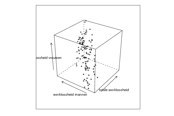
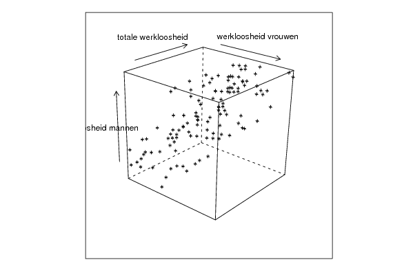
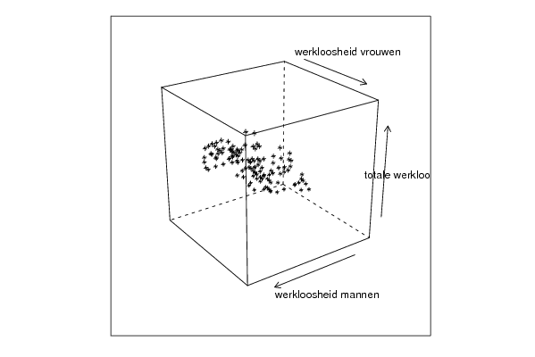
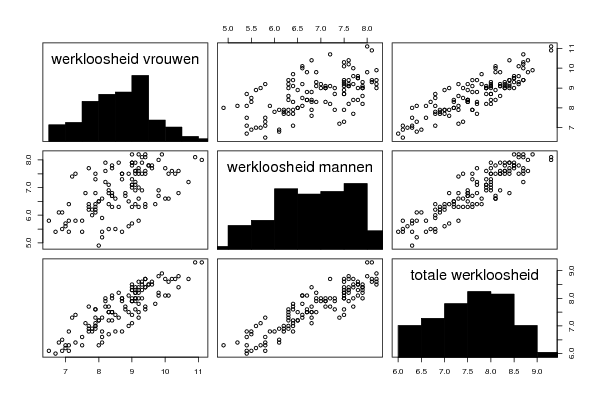
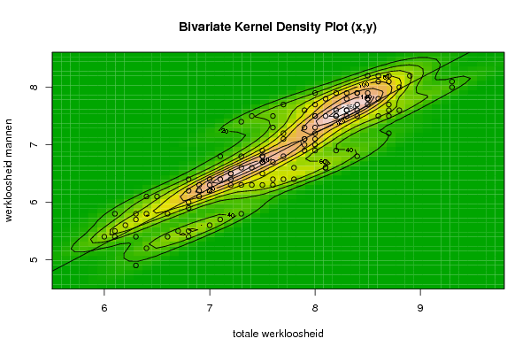
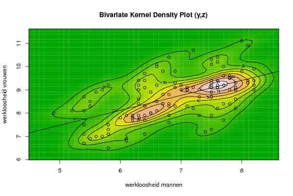
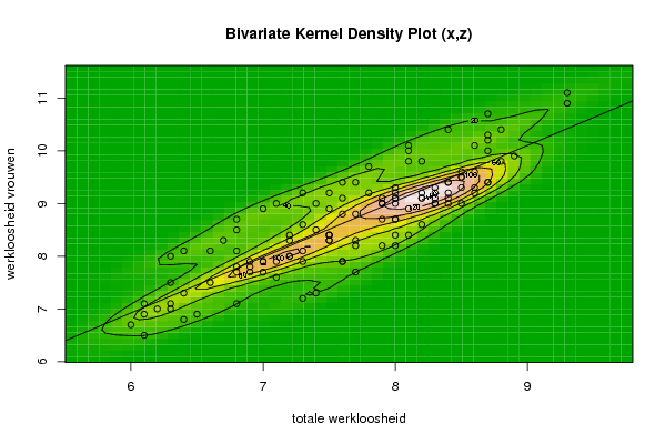
| Title produced by software | Trivariate Scatterplots | ||||||||||||||||||||
| Date of computation | Tue, 03 Nov 2009 12:37:26 -0700 | ||||||||||||||||||||
| Cite this page as follows | Statistical Computations at FreeStatistics.org, Office for Research Development and Education, URL https://freestatistics.org/blog/index.php?v=date/2009/Nov/03/t12572782791138fks99jlnhok.htm/, Retrieved Wed, 01 May 2024 16:45:14 +0000 | ||||||||||||||||||||
| Statistical Computations at FreeStatistics.org, Office for Research Development and Education, URL https://freestatistics.org/blog/index.php?pk=53376, Retrieved Wed, 01 May 2024 16:45:14 +0000 | |||||||||||||||||||||
| QR Codes: | |||||||||||||||||||||
|
| |||||||||||||||||||||
| Original text written by user: | |||||||||||||||||||||
| IsPrivate? | No (this computation is public) | ||||||||||||||||||||
| User-defined keywords | |||||||||||||||||||||
| Estimated Impact | 124 | ||||||||||||||||||||
Tree of Dependent Computations | |||||||||||||||||||||
| Family? (F = Feedback message, R = changed R code, M = changed R Module, P = changed Parameters, D = changed Data) | |||||||||||||||||||||
| - [Trivariate Scatterplots] [workshop5] [2009-11-03 19:37:26] [58c0e7ecdfec19fc38e879e32991032d] [Current] | |||||||||||||||||||||
| Feedback Forum | |||||||||||||||||||||
Post a new message | |||||||||||||||||||||
Dataset | |||||||||||||||||||||
| Dataseries X: | |||||||||||||||||||||
7,4 7,3 7,7 8 8 7,7 6,9 6,6 6,9 7,5 7,9 7,7 6,5 6,1 6,4 6,8 7,1 7,3 7,2 7 7 7 7,3 7,5 7,2 7,7 8 7,9 8 8 7,9 7,9 8 8,1 8,1 8,2 8 8,3 8,5 8,6 8,7 8,7 8,5 8,4 8,5 8,7 8,7 8,6 7,9 8,1 8,2 8,5 8,6 8,5 8,3 8,2 8,7 9,3 9,3 8,8 7,4 7,2 7,5 8,3 8,8 8,9 8,6 8,4 8,4 8,4 8,4 8,3 7,6 7,6 7,9 8 8,2 8,3 8,2 8,1 8 7,8 7,6 7,5 6,8 6,9 7,1 7,3 7,4 7,6 7,6 7,5 7,5 6,8 6,4 6,2 6 6,3 6,3 6,1 6,1 6,3 6,6 6,8 7 7,1 7,3 6,8 6,3 6,4 6,7 6,8 7,2 7,5 7,7 7,8 8,1 8,4 8,7 | |||||||||||||||||||||
| Dataseries Y: | |||||||||||||||||||||
7,5 7,4 7,7 7,9 7,7 7,1 6,2 5,8 6,1 6,9 7,3 7,2 6,1 5,8 6,1 6,4 6,8 6,8 6,5 6,2 6,3 6,4 6,6 6,7 6,4 6,8 7 6,9 7,1 7,2 7,1 7 6,9 6,7 6,6 6,9 7,3 7,9 8,2 8,2 8,2 8,1 7,9 7,7 7,7 7,6 7,5 7,5 7,1 7,5 7,5 7,8 7,8 7,8 7,6 7,5 7,7 8,1 8 7,6 6,6 6,5 6,8 7,5 8 8,2 8,1 7,9 7,9 7,6 7,5 7,6 7,3 7,5 7,6 7,5 7,6 7,8 7,9 7,8 7,5 6,6 6,3 6,3 6 6,3 6,4 6,3 6,3 6,4 6,7 6,7 6,8 6,2 5,8 5,6 5,4 5,7 5,8 5,5 5,4 5,4 5,4 5,5 5,6 5,7 5,8 5,4 4,9 5,2 5,5 5,9 6,3 6,5 6,4 6,4 6,6 6,8 7,2 | |||||||||||||||||||||
| Dataseries Z: | |||||||||||||||||||||
7,3 7,2 7,7 8,2 8,4 8,3 7,8 7,5 7,9 8,3 8,7 8,2 6,9 6,5 6,8 7,1 7,6 7,9 8 7,9 7,9 7,7 8,1 8,4 8,3 8,8 9,2 9,1 9,1 9,1 9 9 9,3 9,8 10 9,8 9 9 9 9,2 9,4 9,4 9,3 9,2 9,6 10,2 10,3 10,1 9 8,9 9,1 9,5 9,6 9,5 9,2 9,2 10 10,9 11,1 10,4 8,5 8 8,3 9,3 9,8 9,9 9,3 9 9,1 9,4 9,4 9,1 7,9 7,9 8,2 8,7 9,1 9 8,6 8,4 8,7 9,2 9,4 9,2 7,8 7,7 7,9 8,6 9 9,1 8,8 8,4 8,4 7,7 7,3 7 6,7 7 7,1 6,9 7,1 7,5 8,1 8,5 8,9 9 9,2 8,7 8 8,1 8,3 8,1 8,4 8,9 9,4 9,7 10,1 10,4 10,7 | |||||||||||||||||||||
Tables (Output of Computation) | |||||||||||||||||||||
| |||||||||||||||||||||
Figures (Output of Computation) | |||||||||||||||||||||
Input Parameters & R Code | |||||||||||||||||||||
| Parameters (Session): | |||||||||||||||||||||
| par1 = 50 ; par2 = 50 ; par3 = Y ; par4 = Y ; par5 = totale werkloosheid ; par6 = werkloosheid mannen ; par7 = werkloosheid vrouwen ; | |||||||||||||||||||||
| Parameters (R input): | |||||||||||||||||||||
| par1 = 50 ; par2 = 50 ; par3 = Y ; par4 = Y ; par5 = totale werkloosheid ; par6 = werkloosheid mannen ; par7 = werkloosheid vrouwen ; | |||||||||||||||||||||
| R code (references can be found in the software module): | |||||||||||||||||||||
x <- array(x,dim=c(length(x),1)) | |||||||||||||||||||||