Free Statistics
of Irreproducible Research!
Description of Statistical Computation | |||||||||||||||||||||||||||||||||||||||||||||||||||||||||||||||||
|---|---|---|---|---|---|---|---|---|---|---|---|---|---|---|---|---|---|---|---|---|---|---|---|---|---|---|---|---|---|---|---|---|---|---|---|---|---|---|---|---|---|---|---|---|---|---|---|---|---|---|---|---|---|---|---|---|---|---|---|---|---|---|---|---|---|
| Author's title | |||||||||||||||||||||||||||||||||||||||||||||||||||||||||||||||||
| Author | *The author of this computation has been verified* | ||||||||||||||||||||||||||||||||||||||||||||||||||||||||||||||||
| R Software Module | rwasp_edabi.wasp | ||||||||||||||||||||||||||||||||||||||||||||||||||||||||||||||||
| Title produced by software | Bivariate Explorative Data Analysis | ||||||||||||||||||||||||||||||||||||||||||||||||||||||||||||||||
| Date of computation | Tue, 03 Nov 2009 12:58:27 -0700 | ||||||||||||||||||||||||||||||||||||||||||||||||||||||||||||||||
| Cite this page as follows | Statistical Computations at FreeStatistics.org, Office for Research Development and Education, URL https://freestatistics.org/blog/index.php?v=date/2009/Nov/03/t1257278402a5sbvni9kszg91h.htm/, Retrieved Wed, 01 May 2024 16:09:00 +0000 | ||||||||||||||||||||||||||||||||||||||||||||||||||||||||||||||||
| Statistical Computations at FreeStatistics.org, Office for Research Development and Education, URL https://freestatistics.org/blog/index.php?pk=53377, Retrieved Wed, 01 May 2024 16:09:00 +0000 | |||||||||||||||||||||||||||||||||||||||||||||||||||||||||||||||||
| QR Codes: | |||||||||||||||||||||||||||||||||||||||||||||||||||||||||||||||||
|
| |||||||||||||||||||||||||||||||||||||||||||||||||||||||||||||||||
| Original text written by user: | WS 5 | ||||||||||||||||||||||||||||||||||||||||||||||||||||||||||||||||
| IsPrivate? | No (this computation is public) | ||||||||||||||||||||||||||||||||||||||||||||||||||||||||||||||||
| User-defined keywords | |||||||||||||||||||||||||||||||||||||||||||||||||||||||||||||||||
| Estimated Impact | 129 | ||||||||||||||||||||||||||||||||||||||||||||||||||||||||||||||||
Tree of Dependent Computations | |||||||||||||||||||||||||||||||||||||||||||||||||||||||||||||||||
| Family? (F = Feedback message, R = changed R code, M = changed R Module, P = changed Parameters, D = changed Data) | |||||||||||||||||||||||||||||||||||||||||||||||||||||||||||||||||
| - [Bivariate Explorative Data Analysis] [WS 5 Y[t] - g - h...] [2009-11-03 19:58:27] [9b6f46453e60f88d91cef176fe926003] [Current] | |||||||||||||||||||||||||||||||||||||||||||||||||||||||||||||||||
| Feedback Forum | |||||||||||||||||||||||||||||||||||||||||||||||||||||||||||||||||
Post a new message | |||||||||||||||||||||||||||||||||||||||||||||||||||||||||||||||||
Dataset | |||||||||||||||||||||||||||||||||||||||||||||||||||||||||||||||||
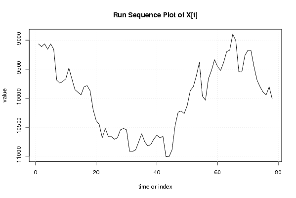
| Dataseries X: | |||||||||||||||||||||||||||||||||||||||||||||||||||||||||||||||||
-9063,91 -9110,33 -9062,71 -9155,95 -9063,71 -9155,85 -9688,93 -9738,65 -9710,89 -9664,17 -9480,59 -9665,97 -9851,55 -9897,17 -9940,89 -9803,43 -9781,27 -9871,41 -10197,65 -10384,93 -10450,51 -10682,01 -10520,39 -10660,05 -10660,75 -10706,47 -10680,81 -10543,15 -10520,59 -10542,35 -10915,21 -10916,41 -10889,15 -10751,69 -10611,33 -10751,39 -10821,37 -10797,91 -10701,97 -10636,39 -10680,51 -10656,95 -11006,55 -11007,95 -10888,85 -10471,57 -10239,87 -10219,41 -10264,13 -10125,47 -9867,91 -9801,23 -9614,75 -9382,15 -9962,35 -10033,73 -9661,07 -9519,71 -9335,93 -9454,53 -9521,01 -9381,75 -9196,27 -9171,51 -8895,29 -9008,49 -9542,67 -9546,77 -9264,35 -9172,21 -9176,71 -9456,03 -9688,03 -9803,43 -9894,77 -9942,19 -9803,63 -10009,97 | |||||||||||||||||||||||||||||||||||||||||||||||||||||||||||||||||
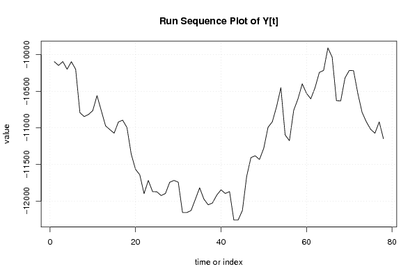
| Dataseries Y: | |||||||||||||||||||||||||||||||||||||||||||||||||||||||||||||||||
-10095,16 -10146,94 -10094,36 -10198,42 -10095,96 -10198,62 -10792,49 -10845,67 -10817,18 -10764,6 -10559,78 -10765,3 -10972,32 -11023,5 -11072,48 -10919,54 -10894,85 -10994,81 -11358,87 -11565,29 -11640,46 -11898,26 -11717,83 -11872,27 -11873,47 -11924,35 -11896,56 -11743,32 -11717,93 -11741,92 -12157,76 -12157,16 -12128,97 -11975,53 -11818,69 -11973,33 -12051,6 -12026,11 -11919,25 -11846,28 -11896,26 -11870,17 -12259,62 -12259,12 -12128,47 -11663,55 -11405,55 -11381,56 -11432,14 -11277,9 -10991,91 -10916,84 -10709,02 -10450,82 -11096,27 -11175,04 -10761 -10603,46 -10398,04 -10528,59 -10603,26 -10449,82 -10242,2 -10215,11 -9907,63 -10033,78 -10628,45 -10630,95 -10318,07 -10215,31 -10219,01 -10530,09 -10788,69 -10918,14 -11019,9 -11073,18 -10918,94 -11148,65 | |||||||||||||||||||||||||||||||||||||||||||||||||||||||||||||||||
Tables (Output of Computation) | |||||||||||||||||||||||||||||||||||||||||||||||||||||||||||||||||
| |||||||||||||||||||||||||||||||||||||||||||||||||||||||||||||||||
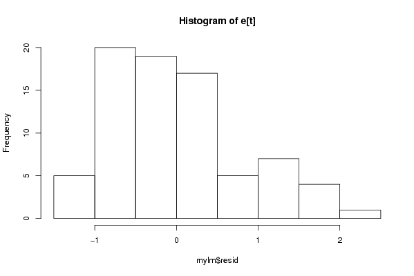
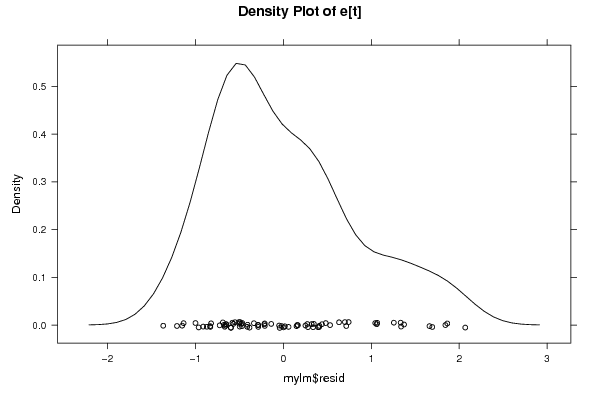
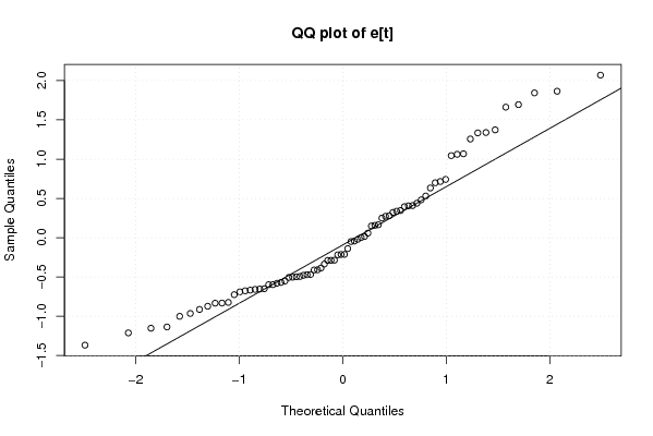
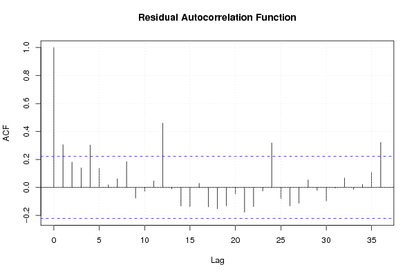
Figures (Output of Computation) | |||||||||||||||||||||||||||||||||||||||||||||||||||||||||||||||||
Input Parameters & R Code | |||||||||||||||||||||||||||||||||||||||||||||||||||||||||||||||||
| Parameters (Session): | |||||||||||||||||||||||||||||||||||||||||||||||||||||||||||||||||
| par1 = 0 ; par2 = 36 ; | |||||||||||||||||||||||||||||||||||||||||||||||||||||||||||||||||
| Parameters (R input): | |||||||||||||||||||||||||||||||||||||||||||||||||||||||||||||||||
| par1 = 0 ; par2 = 36 ; | |||||||||||||||||||||||||||||||||||||||||||||||||||||||||||||||||
| R code (references can be found in the software module): | |||||||||||||||||||||||||||||||||||||||||||||||||||||||||||||||||
par1 <- as.numeric(par1) | |||||||||||||||||||||||||||||||||||||||||||||||||||||||||||||||||