Repository of Reproducible Computations

Free Statistics

of Irreproducible Research!

Author's title

Author

*The author of this computation has been verified*

R Software Module

rwasp_bidensity.wasp

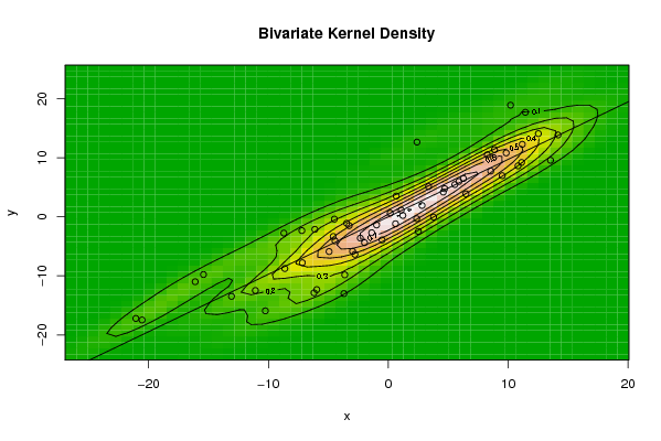
Title produced by software

Bivariate Kernel Density Estimation

Date of computation

Tue, 03 Nov 2009 13:57:11 -0700

Cite this page as follows

Statistical Computations at FreeStatistics.org, Office for Research Development and Education, URL https://freestatistics.org/blog/index.php?v=date/2009/Nov/03/t12572818723ga1qeccql2u3mi.htm/, Retrieved Wed, 01 May 2024 21:07:55 +0000

Statistical Computations at FreeStatistics.org, Office for Research Development and Education, URL https://freestatistics.org/blog/index.php?pk=53416, Retrieved Wed, 01 May 2024 21:07:55 +0000

QR Codes:

Paste this QR Code to cite your computation.

Original text written by user:

IsPrivate?

No (this computation is public)

User-defined keywords

Estimated Impact

150

Family? (F = Feedback message, R = changed R code, M = changed R Module, P = changed Parameters, D = changed Data)

-     [Bivariate Explorative Data Analysis] [WS 5.6] [2009-10-28 16:01:32] [83058a88a37d754675a5cd22dab372fc]
- RMP     [Bivariate Kernel Density Estimation] [WS 5.7] [2009-11-03 20:57:11] [eba9f01697e64705b70041e6f338cb22] [Current]
- RMPD      [Kendall tau Rank Correlation] [WS 5.8] [2009-11-03 20:59:58] [83058a88a37d754675a5cd22dab372fc] 

Feedback Forum

Post a new message

Dataseries X:

Download CSV

Histogram

Boxplots

2,366550914
-2,784331965
11,17687724
-13,08690014
-3,702416453
13,53551828
9,502773534
2,81572168
0,60106142
-7,213545194
-6,130773624
2,389932679
0,66061216
-3,473042289
12,52091167
-20,54891176
-6,198884935
11,12267743
3,776128477
6,474416363
-0,522105764
-4,597921587
-3,270313182
11,43658892
-4,449553233
3,353978285
8,860826741
-21,06844013
-5,968440133
8,548788298
9,837605911
6,268638544
-4,941687785
-0,980478576
-1,983046747
10,82647717
-2,982939457
0,162753436
8,784262151
-16,11744996
-3,633875981
4,70491481
14,16269979
5,551463759
-7,174432532
1,213636315
2,506787859
-1,385400337
5,889613074
-2,333661401
4,590469131
-15,42590324
-10,26046739
8,260131619
10,20132965
-4,500489758
-8,71605972
-11,09283889
-8,636819669
1,076984534

Dataseries Y:

Download CSV

Histogram

-0,3160103
-6,358448377
12,27737808
-13,46500204
-12,99867146
9,566650862
6,96160958
1,918725333
-1,176092864
-2,333737351
-2,125109214
12,64884125
3,499204854
-1,09186136
14,07900638
-17,46250601
-12,86891915
9,203882529
-0,057125727
3,885171829
-3,922249573
-3,325720513
-1,493786564
17,69419692
-4,072662393
5,117089915
11,37789969
-17,20456299
-12,32456299
7,746808873
10,81456927
6,481908112
-5,881480264
-1,385653811
-4,382207478
8,629503386
-5,827860058
0,624296976
10,00992495
-10,98777749
-9,827471845
4,766701702
13,85712327
5,457709958
-7,776521546
0,226735053
-2,474074724
-2,690066305
5,981727122
-3,608777006
4,190578344
-9,771942297
-15,91903344
10,5005696
18,89977568
-0,392274179
-2,763117308
-12,47978689
-8,764241479
1,111725495

Summary of computational transaction
Raw Input	view raw input (R code)
Raw Output	view raw output of R engine
Computing time	1 seconds
R Server	'Gwilym Jenkins' @ 72.249.127.135

\begin{tabular}{lllllllll}
\hline
Summary of computational transaction \tabularnewline
Raw Input & view raw input (R code)  \tabularnewline
Raw Output & view raw output of R engine  \tabularnewline
Computing time & 1 seconds \tabularnewline
R Server & 'Gwilym Jenkins' @ 72.249.127.135 \tabularnewline
\hline
\end{tabular}
%Source: https://freestatistics.org/blog/index.php?pk=53416&T=0

[TABLE]
[ROW][C]Summary of computational transaction[/C][/ROW]
[ROW][C]Raw Input[/C][C]view raw input (R code) [/C][/ROW]
[ROW][C]Raw Output[/C][C]view raw output of R engine [/C][/ROW]
[ROW][C]Computing time[/C][C]1 seconds[/C][/ROW]
[ROW][C]R Server[/C][C]'Gwilym Jenkins' @ 72.249.127.135[/C][/ROW]
[/TABLE]
Source: https://freestatistics.org/blog/index.php?pk=53416&T=0

Globally Unique Identifier (entire table): ba.freestatistics.org/blog/index.php?pk=53416&T=0

As an alternative you can also use a QR Code:

The GUIDs for individual cells are displayed in the table below:

Summary of computational transaction
Raw Input	view raw input (R code)
Raw Output	view raw output of R engine
Computing time	1 seconds
R Server	'Gwilym Jenkins' @ 72.249.127.135

Bandwidth
x axis	3.62002270282313
y axis	4.19027635200873
Correlation
correlation used in KDE	0.910880072263688
correlation(x,y)	0.910880072263688

\begin{tabular}{lllllllll}
\hline
Bandwidth \tabularnewline
x axis & 3.62002270282313 \tabularnewline
y axis & 4.19027635200873 \tabularnewline
Correlation \tabularnewline
correlation used in KDE & 0.910880072263688 \tabularnewline
correlation(x,y) & 0.910880072263688 \tabularnewline
\hline
\end{tabular}
%Source: https://freestatistics.org/blog/index.php?pk=53416&T=1

[TABLE]
[ROW][C]Bandwidth[/C][/ROW]
[ROW][C]x axis[/C][C]3.62002270282313[/C][/ROW]
[ROW][C]y axis[/C][C]4.19027635200873[/C][/ROW]
[ROW][C]Correlation[/C][/ROW]
[ROW][C]correlation used in KDE[/C][C]0.910880072263688[/C][/ROW]
[ROW][C]correlation(x,y)[/C][C]0.910880072263688[/C][/ROW]
[/TABLE]
Source: https://freestatistics.org/blog/index.php?pk=53416&T=1

Globally Unique Identifier (entire table): ba.freestatistics.org/blog/index.php?pk=53416&T=1

As an alternative you can also use a QR Code:

The GUIDs for individual cells are displayed in the table below:

Bandwidth
x axis	3.62002270282313
y axis	4.19027635200873
Correlation
correlation used in KDE	0.910880072263688
correlation(x,y)	0.910880072263688

Figure 1

PNG link

Postscript link

PDF link

Parameters (Session):

par1 = 50 ; par2 = 50 ; par3 = 0 ; par4 = 0 ; par5 = 0 ; par6 = Y ; par7 = Y ;

Parameters (R input):

par1 = 50 ; par2 = 50 ; par3 = 0 ; par4 = 0 ; par5 = 0 ; par6 = Y ; par7 = Y ;

R code (references can be found in the software module):

par1 <- as(par1,'numeric')
par2 <- as(par2,'numeric')
par3 <- as(par3,'numeric')
par4 <- as(par4,'numeric')
par5 <- as(par5,'numeric')
library('GenKern')
if (par3==0) par3 <- dpik(x)
if (par4==0) par4 <- dpik(y)
if (par5==0) par5 <- cor(x,y)
if (par1 > 500) par1 <- 500
if (par2 > 500) par2 <- 500
bitmap(file='bidensity.png')
op <- KernSur(x,y, xgridsize=par1, ygridsize=par2, correlation=par5, xbandwidth=par3, ybandwidth=par4)
image(op$xords, op$yords, op$zden, col=terrain.colors(100), axes=TRUE,main=main,xlab=xlab,ylab=ylab)
if (par6=='Y') contour(op$xords, op$yords, op$zden, add=TRUE)
if (par7=='Y') points(x,y)
(r<-lm(y ~ x))
abline(r)
box()
dev.off()
load(file='createtable')
a<-table.start()
a<-table.row.start(a)
a<-table.element(a,'Bandwidth',2,TRUE)
a<-table.row.end(a)
a<-table.row.start(a)
a<-table.element(a,'x axis',header=TRUE)
a<-table.element(a,par3)
a<-table.row.end(a)
a<-table.row.start(a)
a<-table.element(a,'y axis',header=TRUE)
a<-table.element(a,par4)
a<-table.row.end(a)
a<-table.row.start(a)
a<-table.element(a,'Correlation',2,TRUE)
a<-table.row.end(a)
a<-table.row.start(a)
a<-table.element(a,'correlation used in KDE',header=TRUE)
a<-table.element(a,par5)
a<-table.row.end(a)
a<-table.row.start(a)
a<-table.element(a,'correlation(x,y)',header=TRUE)
a<-table.element(a,cor(x,y))
a<-table.row.end(a)
a<-table.end(a)
table.save(a,file='mytable.tab')

Free Statistics

Description of Statistical Computation

Tree of Dependent Computations

Dataset

Tables (Output of Computation)

Figures (Output of Computation)

Input Parameters & R Code