Free Statistics
of Irreproducible Research!
Description of Statistical Computation | |||||||||||||||||||||||||||||||||||||||||||||||||||||||||||||||||
|---|---|---|---|---|---|---|---|---|---|---|---|---|---|---|---|---|---|---|---|---|---|---|---|---|---|---|---|---|---|---|---|---|---|---|---|---|---|---|---|---|---|---|---|---|---|---|---|---|---|---|---|---|---|---|---|---|---|---|---|---|---|---|---|---|---|
| Author's title | |||||||||||||||||||||||||||||||||||||||||||||||||||||||||||||||||
| Author | *The author of this computation has been verified* | ||||||||||||||||||||||||||||||||||||||||||||||||||||||||||||||||
| R Software Module | rwasp_edabi.wasp | ||||||||||||||||||||||||||||||||||||||||||||||||||||||||||||||||
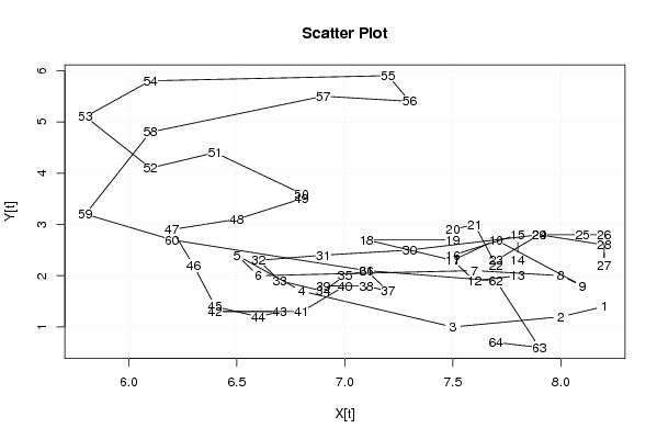
| Title produced by software | Bivariate Explorative Data Analysis | ||||||||||||||||||||||||||||||||||||||||||||||||||||||||||||||||
| Date of computation | Tue, 03 Nov 2009 14:45:54 -0700 | ||||||||||||||||||||||||||||||||||||||||||||||||||||||||||||||||
| Cite this page as follows | Statistical Computations at FreeStatistics.org, Office for Research Development and Education, URL https://freestatistics.org/blog/index.php?v=date/2009/Nov/03/t1257284880ecq0lostx3imjit.htm/, Retrieved Wed, 01 May 2024 14:24:13 +0000 | ||||||||||||||||||||||||||||||||||||||||||||||||||||||||||||||||
| Statistical Computations at FreeStatistics.org, Office for Research Development and Education, URL https://freestatistics.org/blog/index.php?pk=53441, Retrieved Wed, 01 May 2024 14:24:13 +0000 | |||||||||||||||||||||||||||||||||||||||||||||||||||||||||||||||||
| QR Codes: | |||||||||||||||||||||||||||||||||||||||||||||||||||||||||||||||||
|
| |||||||||||||||||||||||||||||||||||||||||||||||||||||||||||||||||
| Original text written by user: | |||||||||||||||||||||||||||||||||||||||||||||||||||||||||||||||||
| IsPrivate? | No (this computation is public) | ||||||||||||||||||||||||||||||||||||||||||||||||||||||||||||||||
| User-defined keywords | ws5 eda 2 | ||||||||||||||||||||||||||||||||||||||||||||||||||||||||||||||||
| Estimated Impact | 174 | ||||||||||||||||||||||||||||||||||||||||||||||||||||||||||||||||
Tree of Dependent Computations | |||||||||||||||||||||||||||||||||||||||||||||||||||||||||||||||||
| Family? (F = Feedback message, R = changed R code, M = changed R Module, P = changed Parameters, D = changed Data) | |||||||||||||||||||||||||||||||||||||||||||||||||||||||||||||||||
| - [Trivariate Scatterplots] [workshop 5] [2009-10-29 16:20:09] [309ee52d0058ff0a6f7eec15e07b2d9f] - MPD [Trivariate Scatterplots] [Workshop 5 xyz] [2009-11-03 20:27:02] [616e2df490b611f6cb7080068870ecbd] - RMP [Partial Correlation] [WS5 Partial Corre...] [2009-11-03 20:34:59] [616e2df490b611f6cb7080068870ecbd] - RMPD [Bivariate Explorative Data Analysis] [WS5 Bivariate EDA] [2009-11-03 21:05:09] [616e2df490b611f6cb7080068870ecbd] - D [Bivariate Explorative Data Analysis] [Workshop 5 Bivari...] [2009-11-03 21:45:54] [88e98f4c87ea17c4967db8279bda8533] [Current] - D [Bivariate Explorative Data Analysis] [WS5 Bivariate EDA...] [2009-11-03 21:59:14] [616e2df490b611f6cb7080068870ecbd] | |||||||||||||||||||||||||||||||||||||||||||||||||||||||||||||||||
| Feedback Forum | |||||||||||||||||||||||||||||||||||||||||||||||||||||||||||||||||
Post a new message | |||||||||||||||||||||||||||||||||||||||||||||||||||||||||||||||||
Dataset | |||||||||||||||||||||||||||||||||||||||||||||||||||||||||||||||||
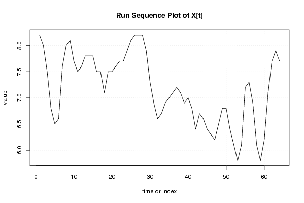
| Dataseries X: | |||||||||||||||||||||||||||||||||||||||||||||||||||||||||||||||||
8.2 8 7.5 6.8 6.5 6.6 7.6 8 8.1 7.7 7.5 7.6 7.8 7.8 7.8 7.5 7.5 7.1 7.5 7.5 7.6 7.7 7.7 7.9 8.1 8.2 8.2 8.2 7.9 7.3 6.9 6.6 6.7 6.9 7 7.1 7.2 7.1 6.9 7 6.8 6.4 6.7 6.6 6.4 6.3 6.2 6.5 6.8 6.8 6.4 6.1 5.8 6.1 7.2 7.3 6.9 6.1 5.8 6.2 7.1 7.7 7.9 7.7 | |||||||||||||||||||||||||||||||||||||||||||||||||||||||||||||||||
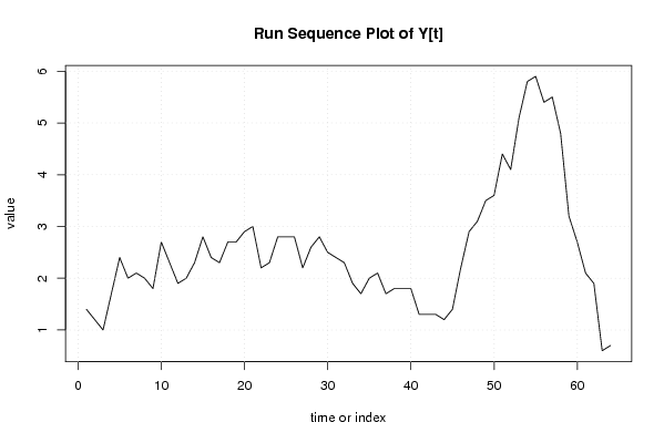
| Dataseries Y: | |||||||||||||||||||||||||||||||||||||||||||||||||||||||||||||||||
1.4 1.2 1.0 1.7 2.4 2.0 2.1 2.0 1.8 2.7 2.3 1.9 2.0 2.3 2.8 2.4 2.3 2.7 2.7 2.9 3.0 2.2 2.3 2.8 2.8 2.8 2.2 2.6 2.8 2.5 2.4 2.3 1.9 1.7 2.0 2.1 1.7 1.8 1.8 1.8 1.3 1.3 1.3 1.2 1.4 2.2 2.9 3.1 3.5 3.6 4.4 4.1 5.1 5.8 5.9 5.4 5.5 4.8 3.2 2.7 2.1 1.9 0.6 0.7 | |||||||||||||||||||||||||||||||||||||||||||||||||||||||||||||||||
Tables (Output of Computation) | |||||||||||||||||||||||||||||||||||||||||||||||||||||||||||||||||
| |||||||||||||||||||||||||||||||||||||||||||||||||||||||||||||||||
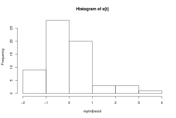
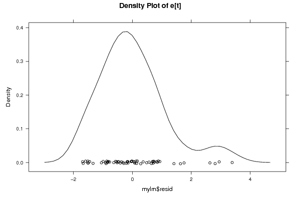
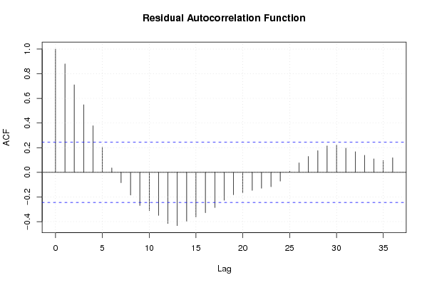
Figures (Output of Computation) | |||||||||||||||||||||||||||||||||||||||||||||||||||||||||||||||||
Input Parameters & R Code | |||||||||||||||||||||||||||||||||||||||||||||||||||||||||||||||||
| Parameters (Session): | |||||||||||||||||||||||||||||||||||||||||||||||||||||||||||||||||
| par1 = 0 ; par2 = 36 ; | |||||||||||||||||||||||||||||||||||||||||||||||||||||||||||||||||
| Parameters (R input): | |||||||||||||||||||||||||||||||||||||||||||||||||||||||||||||||||
| par1 = 0 ; par2 = 36 ; | |||||||||||||||||||||||||||||||||||||||||||||||||||||||||||||||||
| R code (references can be found in the software module): | |||||||||||||||||||||||||||||||||||||||||||||||||||||||||||||||||
par1 <- as.numeric(par1) | |||||||||||||||||||||||||||||||||||||||||||||||||||||||||||||||||