Free Statistics
of Irreproducible Research!
Description of Statistical Computation | |||||||||||||||||||||
|---|---|---|---|---|---|---|---|---|---|---|---|---|---|---|---|---|---|---|---|---|---|
| Author's title | |||||||||||||||||||||
| Author | *The author of this computation has been verified* | ||||||||||||||||||||
| R Software Module | rwasp_cloud.wasp | ||||||||||||||||||||
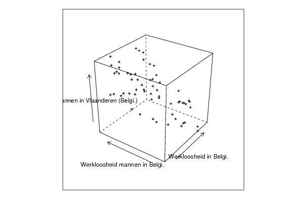
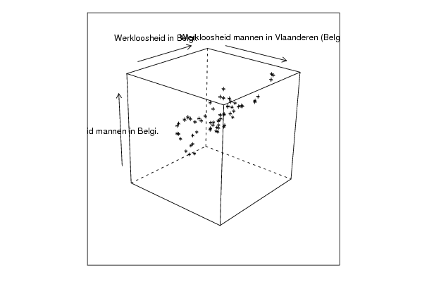
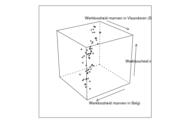
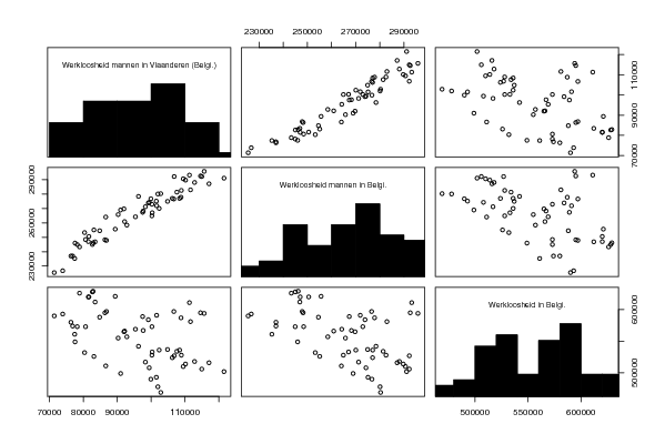
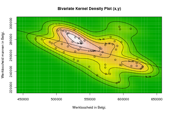
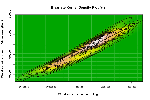
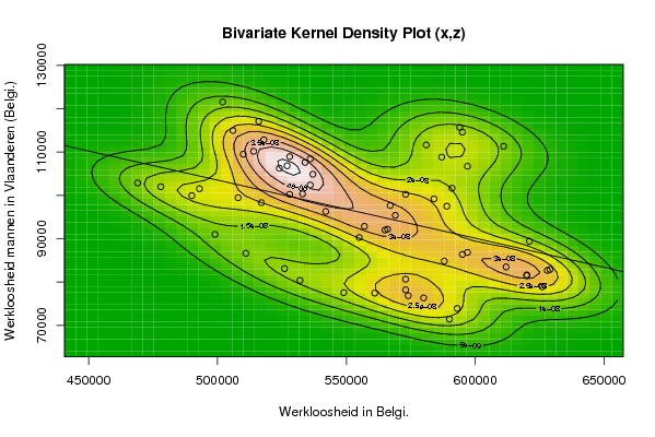
| Title produced by software | Trivariate Scatterplots | ||||||||||||||||||||
| Date of computation | Tue, 03 Nov 2009 17:35:18 -0700 | ||||||||||||||||||||
| Cite this page as follows | Statistical Computations at FreeStatistics.org, Office for Research Development and Education, URL https://freestatistics.org/blog/index.php?v=date/2009/Nov/04/t1257294992hqeuyux9b74iyl7.htm/, Retrieved Mon, 29 Apr 2024 10:38:56 +0000 | ||||||||||||||||||||
| Statistical Computations at FreeStatistics.org, Office for Research Development and Education, URL https://freestatistics.org/blog/index.php?pk=53472, Retrieved Mon, 29 Apr 2024 10:38:56 +0000 | |||||||||||||||||||||
| QR Codes: | |||||||||||||||||||||
|
| |||||||||||||||||||||
| Original text written by user: | |||||||||||||||||||||
| IsPrivate? | No (this computation is public) | ||||||||||||||||||||
| User-defined keywords | |||||||||||||||||||||
| Estimated Impact | 161 | ||||||||||||||||||||
Tree of Dependent Computations | |||||||||||||||||||||
| Family? (F = Feedback message, R = changed R code, M = changed R Module, P = changed Parameters, D = changed Data) | |||||||||||||||||||||
| - [Trivariate Scatterplots] [Trivariate scatte...] [2009-10-29 19:06:49] [214e6e00abbde49700521a7ef1d30da2] - RMPD [Trivariate Scatterplots] [WorkShop5 (SHW)] [2009-11-04 00:35:18] [2d9a0b3c2f25bb8f387fafb994d0d852] [Current] | |||||||||||||||||||||
| Feedback Forum | |||||||||||||||||||||
Post a new message | |||||||||||||||||||||
Dataset | |||||||||||||||||||||
| Dataseries X: | |||||||||||||||||||||
581000 597000 587000 536000 524000 537000 536000 533000 528000 516000 502000 506000 518000 534000 528000 478000 469000 490000 493000 508000 517000 514000 510000 527000 542000 565000 555000 499000 511000 526000 532000 549000 561000 557000 566000 588000 620000 626000 620000 573000 573000 574000 580000 590000 593000 597000 595000 612000 628000 629000 621000 569000 567000 573000 584000 589000 591000 595000 594000 611000 | |||||||||||||||||||||
| Dataseries Y: | |||||||||||||||||||||
282965 276610 277838 277051 277026 274960 270073 267063 264916 287182 291109 292223 288109 281400 282579 280113 280331 276759 275139 274275 271234 289725 290649 292223 278429 269749 265784 268957 264099 255121 253276 245980 235295 258479 260916 254586 250566 243345 247028 248464 244962 237003 237008 225477 226762 247857 248256 246892 245021 246186 255688 264242 268270 272969 273886 267353 271916 292633 295804 293222 | |||||||||||||||||||||
| Dataseries Z: | |||||||||||||||||||||
111632 106707 108827 108413 106249 104861 102382 100320 100228 117089 121523 114948 112831 107605 108928 101993 102850 99925 101536 99450 98305 110159 109483 106810 96279 91982 90276 90999 86622 83117 80367 77550 77443 92844 92175 84822 81632 78872 81485 80651 78192 76844 76335 71415 73899 86822 86371 83469 82662 82880 89406 95378 97657 100247 99180 97493 101628 114585 115669 111311 | |||||||||||||||||||||
Tables (Output of Computation) | |||||||||||||||||||||
| |||||||||||||||||||||
Figures (Output of Computation) | |||||||||||||||||||||
Input Parameters & R Code | |||||||||||||||||||||
| Parameters (Session): | |||||||||||||||||||||
| par1 = 50 ; par2 = 50 ; par3 = Y ; par4 = Y ; par5 = Werkloosheid in Belgi� ; par6 = Werkloosheid mannen in Belgi� ; par7 = Werkloosheid mannen in Vlaanderen (Belgi�) ; | |||||||||||||||||||||
| Parameters (R input): | |||||||||||||||||||||
| par1 = 50 ; par2 = 50 ; par3 = Y ; par4 = Y ; par5 = Werkloosheid in Belgi� ; par6 = Werkloosheid mannen in Belgi� ; par7 = Werkloosheid mannen in Vlaanderen (Belgi�) ; | |||||||||||||||||||||
| R code (references can be found in the software module): | |||||||||||||||||||||
x <- array(x,dim=c(length(x),1)) | |||||||||||||||||||||