Free Statistics
of Irreproducible Research!
Description of Statistical Computation | |||||||||||||||||||||
|---|---|---|---|---|---|---|---|---|---|---|---|---|---|---|---|---|---|---|---|---|---|
| Author's title | |||||||||||||||||||||
| Author | *The author of this computation has been verified* | ||||||||||||||||||||
| R Software Module | rwasp_cloud.wasp | ||||||||||||||||||||
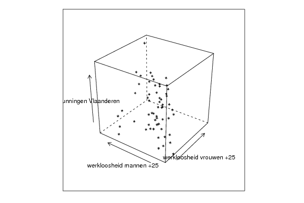
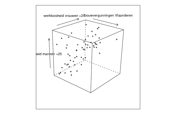
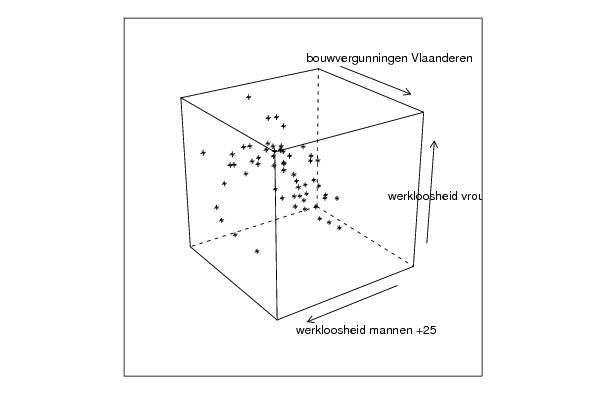
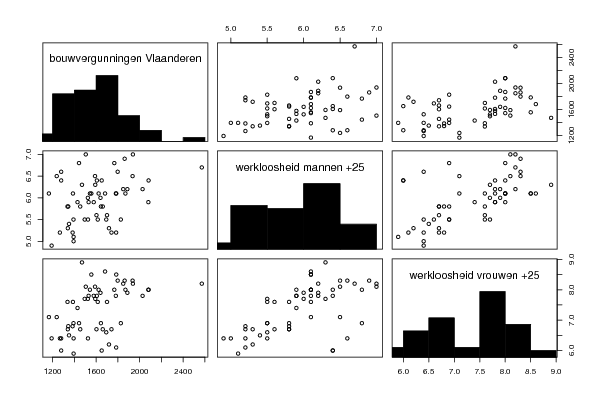
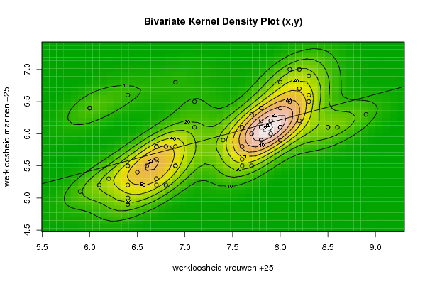
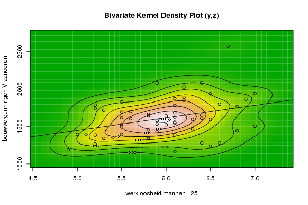
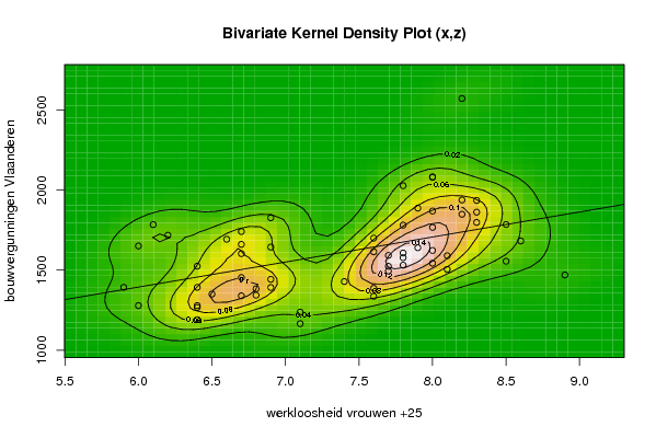
| Title produced by software | Trivariate Scatterplots | ||||||||||||||||||||
| Date of computation | Wed, 04 Nov 2009 03:14:21 -0700 | ||||||||||||||||||||
| Cite this page as follows | Statistical Computations at FreeStatistics.org, Office for Research Development and Education, URL https://freestatistics.org/blog/index.php?v=date/2009/Nov/04/t1257329717l0o0ryu98v3v875.htm/, Retrieved Mon, 29 Apr 2024 12:35:52 +0000 | ||||||||||||||||||||
| Statistical Computations at FreeStatistics.org, Office for Research Development and Education, URL https://freestatistics.org/blog/index.php?pk=53504, Retrieved Mon, 29 Apr 2024 12:35:52 +0000 | |||||||||||||||||||||
| QR Codes: | |||||||||||||||||||||
|
| |||||||||||||||||||||
| Original text written by user: | |||||||||||||||||||||
| IsPrivate? | No (this computation is public) | ||||||||||||||||||||
| User-defined keywords | |||||||||||||||||||||
| Estimated Impact | 165 | ||||||||||||||||||||
Tree of Dependent Computations | |||||||||||||||||||||
| Family? (F = Feedback message, R = changed R code, M = changed R Module, P = changed Parameters, D = changed Data) | |||||||||||||||||||||
| - [Trivariate Scatterplots] [Trivariate scatte...] [2009-11-04 10:14:21] [244731fa3e7e6c85774b8c0902c58f85] [Current] - RMPD [Partial Correlation] [Pearson correlation ] [2009-11-04 10:23:15] [ba905ddf7cdf9ecb063c35348c4dab2e] | |||||||||||||||||||||
| Feedback Forum | |||||||||||||||||||||
Post a new message | |||||||||||||||||||||
Dataset | |||||||||||||||||||||
| Dataseries X: | |||||||||||||||||||||
8,9 8,2 7,6 7,7 8,1 8,3 8,3 7,9 7,8 8 8,5 8,6 8,5 8 7,8 8 8,2 8,3 8,2 8,1 8 7,8 7,8 7,7 7,6 7,6 7,6 7,8 8 8 7,9 7,7 7,4 6,9 6,7 6,5 6,4 6,7 6,8 6,9 6,9 6,7 6,4 6,2 5,9 6,1 6,7 6,8 6,6 6,4 6,4 6,7 7,1 7,1 6,9 6,4 6 6 | |||||||||||||||||||||
| Dataseries Y: | |||||||||||||||||||||
6,3 6,2 6,1 6,3 6,5 6,6 6,5 6,2 6,2 5,9 6,1 6,1 6,1 6,1 6,1 6,4 6,7 6,9 7 7 6,8 6,4 5,9 5,5 5,5 5,6 5,8 5,9 6,1 6,1 6 6 5,9 5,5 5,6 5,4 5,2 5,2 5,2 5,5 5,8 5,8 5,5 5,3 5,1 5,2 5,8 5,8 5,5 5 4,9 5,3 6,1 6,5 6,8 6,6 6,4 6,4 | |||||||||||||||||||||
| Dataseries Z: | |||||||||||||||||||||
1470 1849 1387 1592 1590 1798 1935 1887 2027 2080 1556 1682 1785 1869 1781 2082 2571 1862 1938 1505 1767 1607 1578 1495 1615 1700 1337 1531 1623 1543 1640 1524 1429 1827 1603 1351 1267 1741 1384 1392 1644 1661 1525 1718 1393 1784 1454 1344 1693 1393 1191 1340 1166 1238 1443 1279 1279 1651 | |||||||||||||||||||||
Tables (Output of Computation) | |||||||||||||||||||||
| |||||||||||||||||||||
Figures (Output of Computation) | |||||||||||||||||||||
Input Parameters & R Code | |||||||||||||||||||||
| Parameters (Session): | |||||||||||||||||||||
| par1 = 50 ; par2 = 50 ; par3 = Y ; par4 = Y ; par5 = werkloosheid vrouwen +25 ; par6 = werkloosheid mannen +25 ; par7 = bouwvergunningen Vlaanderen ; | |||||||||||||||||||||
| Parameters (R input): | |||||||||||||||||||||
| par1 = 50 ; par2 = 50 ; par3 = Y ; par4 = Y ; par5 = werkloosheid vrouwen +25 ; par6 = werkloosheid mannen +25 ; par7 = bouwvergunningen Vlaanderen ; | |||||||||||||||||||||
| R code (references can be found in the software module): | |||||||||||||||||||||
x <- array(x,dim=c(length(x),1)) | |||||||||||||||||||||