Repository of Reproducible Computations

Free Statistics

of Irreproducible Research!

Author's title

Author

*The author of this computation has been verified*

R Software Module

rwasp_cloud.wasp

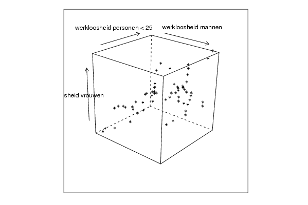
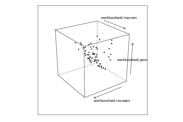
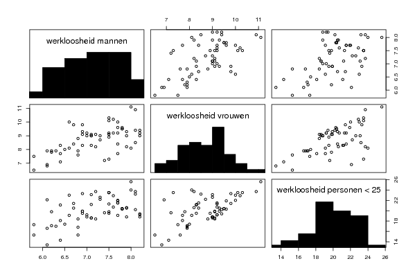
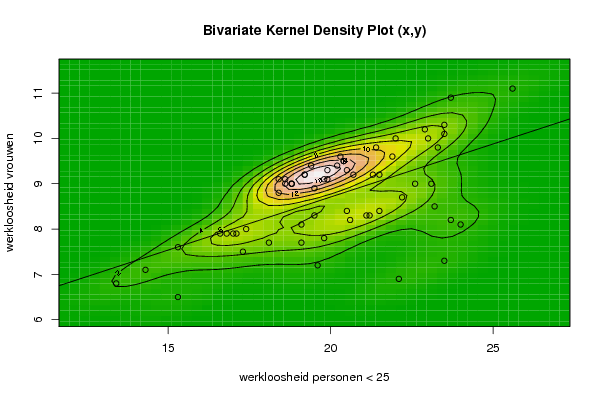
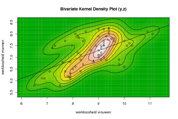
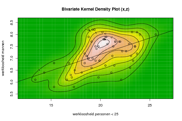
Title produced by software

Trivariate Scatterplots

Date of computation

Wed, 04 Nov 2009 03:45:38 -0700

Cite this page as follows

Statistical Computations at FreeStatistics.org, Office for Research Development and Education, URL https://freestatistics.org/blog/index.php?v=date/2009/Nov/04/t1257331664cvt1ics7w9j0gk1.htm/, Retrieved Mon, 29 Apr 2024 11:38:38 +0000

Statistical Computations at FreeStatistics.org, Office for Research Development and Education, URL https://freestatistics.org/blog/index.php?pk=53526, Retrieved Mon, 29 Apr 2024 11:38:38 +0000

QR Codes:

Paste this QR Code to cite your computation.

Original text written by user:

IsPrivate?

No (this computation is public)

User-defined keywords

Estimated Impact

161

Family? (F = Feedback message, R = changed R code, M = changed R Module, P = changed Parameters, D = changed Data)

-     [Partial Correlation] [workshop 5] [2009-11-03 18:55:39] [0a7d38ad9c7f1a2c46637c75a8a0e083]
- RMPD    [Trivariate Scatterplots] [workshop 5] [2009-11-04 10:45:38] [30a48cc4afddc7f052994dfe2358176d] [Current]

Feedback Forum

Post a new message

Dataseries X:

Download CSV

Histogram

Boxplots

25.6
23.7
22.0
21.3
20.7
20.4
20.3
20.4
19.8
19.5
23.1
23.5
23.5
22.9
21.9
21.5
20.5
20.2
19.4
19.2
18.8
18.8
22.6
23.3
23.0
21.4
19.9
18.8
18.6
18.4
18.6
19.9
19.2
18.4
21.1
20.5
19.1
18.1
17.0
17.1
17.4
16.8
15.3
14.3
13.4
15.3
22.1
23.7
22.2
19.5
16.6
17.3
19.8
21.2
21.5
20.6
19.1
19.6
23.5
24.0
23.2

Dataseries Y:

Download CSV

Histogram

11.1
10.9
10
9.2
9.2
9.5
9.6
9.5
9.1
8.9
9
10.1
10.3
10.2
9.6
9.2
9.3
9.4
9.4
9.2
9
9
9
9.8
10
9.8
9.3
9
9
9.1
9.1
9.1
9.2
8.8
8.3
8.4
8.1
7.7
7.9
7.9
8
7.9
7.6
7.1
6.8
6.5
6.9
8.2
8.7
8.3
7.9
7.5
7.8
8.3
8.4
8.2
7.7
7.2
7.3
8.1
8.5

Dataseries Z:

Download CSV

Histogram

8
8.1
7.7
7.5
7.6
7.8
7.8
7.8
7.5
7.5
7.1
7.5
7.5
7.6
7.7
7.7
7.9
8.1
8.2
8.2
8.2
7.9
7.3
6.9
6.6
6.7
6.9
7
7.1
7.2
7.1
6.9
7
6.8
6.4
6.7
6.6
6.4
6.3
6.2
6.5
6.8
6.8
6.4
6.1
5.8
6.1
7.2
7.3
6.9
6.1
5.8
6.2
7.1
7.7
7.9
7.7
7.4
7.5
8
8.1

Summary of computational transaction
Raw Input	view raw input (R code)
Raw Output	view raw output of R engine
Computing time	5 seconds
R Server	'RServer@AstonUniversity' @ vre.aston.ac.uk

\begin{tabular}{lllllllll}
\hline
Summary of computational transaction \tabularnewline
Raw Input & view raw input (R code)  \tabularnewline
Raw Output & view raw output of R engine  \tabularnewline
Computing time & 5 seconds \tabularnewline
R Server & 'RServer@AstonUniversity' @ vre.aston.ac.uk \tabularnewline
\hline
\end{tabular}
%Source: https://freestatistics.org/blog/index.php?pk=53526&T=0

[TABLE]
[ROW][C]Summary of computational transaction[/C][/ROW]
[ROW][C]Raw Input[/C][C]view raw input (R code) [/C][/ROW]
[ROW][C]Raw Output[/C][C]view raw output of R engine [/C][/ROW]
[ROW][C]Computing time[/C][C]5 seconds[/C][/ROW]
[ROW][C]R Server[/C][C]'RServer@AstonUniversity' @ vre.aston.ac.uk[/C][/ROW]
[/TABLE]
Source: https://freestatistics.org/blog/index.php?pk=53526&T=0

Globally Unique Identifier (entire table): ba.freestatistics.org/blog/index.php?pk=53526&T=0

As an alternative you can also use a QR Code:

The GUIDs for individual cells are displayed in the table below:

Summary of computational transaction
Raw Input	view raw input (R code)
Raw Output	view raw output of R engine
Computing time	5 seconds
R Server	'RServer@AstonUniversity' @ vre.aston.ac.uk

Figure 1

PNG link

Postscript link

PDF link

Figure 2

PNG link

Postscript link

PDF link

Figure 3

PNG link

Postscript link

PDF link

Figure 4

PNG link

Postscript link

PDF link

Figure 5

PNG link

Postscript link

PDF link

Figure 6

PNG link

Postscript link

PDF link

Figure 7

PNG link

Postscript link

PDF link

Parameters (Session):

par1 = 50 ; par2 = 50 ; par3 = Y ; par4 = Y ; par5 = werkloosheid personen < 25 ; par6 = werkloosheid vrouwen ; par7 = werkloosheid mannen ;

Parameters (R input):

par1 = 50 ; par2 = 50 ; par3 = Y ; par4 = Y ; par5 = werkloosheid personen < 25 ; par6 = werkloosheid vrouwen ; par7 = werkloosheid mannen ;

R code (references can be found in the software module):

x <- array(x,dim=c(length(x),1))
colnames(x) <- par5
y <- array(y,dim=c(length(y),1))
colnames(y) <- par6
z <- array(z,dim=c(length(z),1))
colnames(z) <- par7
d <- data.frame(cbind(z,y,x))
colnames(d) <- list(par7,par6,par5)
par1 <- as.numeric(par1)
par2 <- as.numeric(par2)
if (par1>500) par1 <- 500
if (par2>500) par2 <- 500
if (par1<10) par1 <- 10
if (par2<10) par2 <- 10
library(GenKern)
library(lattice)
panel.hist <- function(x, ...)
{
usr <- par('usr'); on.exit(par(usr))
par(usr = c(usr[1:2], 0, 1.5) )
h <- hist(x, plot = FALSE)
breaks <- h$breaks; nB <- length(breaks)
y <- h$counts; y <- y/max(y)
rect(breaks[-nB], 0, breaks[-1], y, col='black', ...)
}
bitmap(file='cloud1.png')
cloud(z~x*y, screen = list(x=-45, y=45, z=35),xlab=par5,ylab=par6,zlab=par7)
dev.off()
bitmap(file='cloud2.png')
cloud(z~x*y, screen = list(x=35, y=45, z=25),xlab=par5,ylab=par6,zlab=par7)
dev.off()
bitmap(file='cloud3.png')
cloud(z~x*y, screen = list(x=35, y=-25, z=90),xlab=par5,ylab=par6,zlab=par7)
dev.off()
bitmap(file='pairs.png')
pairs(d,diag.panel=panel.hist)
dev.off()
x <- as.vector(x)
y <- as.vector(y)
z <- as.vector(z)
bitmap(file='bidensity1.png')
op <- KernSur(x,y, xgridsize=par1, ygridsize=par2, correlation=cor(x,y), xbandwidth=dpik(x), ybandwidth=dpik(y))
image(op$xords, op$yords, op$zden, col=terrain.colors(100), axes=TRUE,main='Bivariate Kernel Density Plot (x,y)',xlab=par5,ylab=par6)
if (par3=='Y') contour(op$xords, op$yords, op$zden, add=TRUE)
if (par4=='Y') points(x,y)
(r<-lm(y ~ x))
abline(r)
box()
dev.off()
bitmap(file='bidensity2.png')
op <- KernSur(y,z, xgridsize=par1, ygridsize=par2, correlation=cor(y,z), xbandwidth=dpik(y), ybandwidth=dpik(z))
op
image(op$xords, op$yords, op$zden, col=terrain.colors(100), axes=TRUE,main='Bivariate Kernel Density Plot (y,z)',xlab=par6,ylab=par7)
if (par3=='Y') contour(op$xords, op$yords, op$zden, add=TRUE)
if (par4=='Y') points(y,z)
(r<-lm(z ~ y))
abline(r)
box()
dev.off()
bitmap(file='bidensity3.png')
op <- KernSur(x,z, xgridsize=par1, ygridsize=par2, correlation=cor(x,z), xbandwidth=dpik(x), ybandwidth=dpik(z))
op
image(op$xords, op$yords, op$zden, col=terrain.colors(100), axes=TRUE,main='Bivariate Kernel Density Plot (x,z)',xlab=par5,ylab=par7)
if (par3=='Y') contour(op$xords, op$yords, op$zden, add=TRUE)
if (par4=='Y') points(x,z)
(r<-lm(z ~ x))
abline(r)
box()
dev.off()

Free Statistics

Description of Statistical Computation

Tree of Dependent Computations

Dataset

Tables (Output of Computation)

Figures (Output of Computation)

Input Parameters & R Code