Free Statistics
of Irreproducible Research!
Description of Statistical Computation | |||||||||||||||||||||||||||||||||||||||||||||||||||||||||||||||||
|---|---|---|---|---|---|---|---|---|---|---|---|---|---|---|---|---|---|---|---|---|---|---|---|---|---|---|---|---|---|---|---|---|---|---|---|---|---|---|---|---|---|---|---|---|---|---|---|---|---|---|---|---|---|---|---|---|---|---|---|---|---|---|---|---|---|
| Author's title | |||||||||||||||||||||||||||||||||||||||||||||||||||||||||||||||||
| Author | *The author of this computation has been verified* | ||||||||||||||||||||||||||||||||||||||||||||||||||||||||||||||||
| R Software Module | rwasp_edabi.wasp | ||||||||||||||||||||||||||||||||||||||||||||||||||||||||||||||||
| Title produced by software | Bivariate Explorative Data Analysis | ||||||||||||||||||||||||||||||||||||||||||||||||||||||||||||||||
| Date of computation | Wed, 04 Nov 2009 03:55:14 -0700 | ||||||||||||||||||||||||||||||||||||||||||||||||||||||||||||||||
| Cite this page as follows | Statistical Computations at FreeStatistics.org, Office for Research Development and Education, URL https://freestatistics.org/blog/index.php?v=date/2009/Nov/04/t1257332206wveew4rujs4mtgk.htm/, Retrieved Mon, 29 Apr 2024 10:00:10 +0000 | ||||||||||||||||||||||||||||||||||||||||||||||||||||||||||||||||
| Statistical Computations at FreeStatistics.org, Office for Research Development and Education, URL https://freestatistics.org/blog/index.php?pk=53538, Retrieved Mon, 29 Apr 2024 10:00:10 +0000 | |||||||||||||||||||||||||||||||||||||||||||||||||||||||||||||||||
| QR Codes: | |||||||||||||||||||||||||||||||||||||||||||||||||||||||||||||||||
|
| |||||||||||||||||||||||||||||||||||||||||||||||||||||||||||||||||
| Original text written by user: | |||||||||||||||||||||||||||||||||||||||||||||||||||||||||||||||||
| IsPrivate? | No (this computation is public) | ||||||||||||||||||||||||||||||||||||||||||||||||||||||||||||||||
| User-defined keywords | WS 5, Bivariate Explorative Data Analysis | ||||||||||||||||||||||||||||||||||||||||||||||||||||||||||||||||
| Estimated Impact | 161 | ||||||||||||||||||||||||||||||||||||||||||||||||||||||||||||||||
Tree of Dependent Computations | |||||||||||||||||||||||||||||||||||||||||||||||||||||||||||||||||
| Family? (F = Feedback message, R = changed R code, M = changed R Module, P = changed Parameters, D = changed Data) | |||||||||||||||||||||||||||||||||||||||||||||||||||||||||||||||||
| - [Bivariate Data Series] [Bivariate dataset] [2008-01-05 23:51:08] [74be16979710d4c4e7c6647856088456] - RMPD [Bivariate Explorative Data Analysis] [] [2009-10-28 15:16:32] [5482608004c1d7bbf873930172393a2d] - D [Bivariate Explorative Data Analysis] [] [2009-10-28 16:44:36] [5482608004c1d7bbf873930172393a2d] - RMPD [Trivariate Scatterplots] [] [2009-11-03 17:57:36] [5482608004c1d7bbf873930172393a2d] - RMPD [Bivariate Explorative Data Analysis] [] [2009-11-03 18:16:45] [5482608004c1d7bbf873930172393a2d] - D [Bivariate Explorative Data Analysis] [Workshop 5, Bivar...] [2009-11-04 10:55:14] [a53416c107f5e7e1e12bb9940270d09d] [Current] | |||||||||||||||||||||||||||||||||||||||||||||||||||||||||||||||||
| Feedback Forum | |||||||||||||||||||||||||||||||||||||||||||||||||||||||||||||||||
Post a new message | |||||||||||||||||||||||||||||||||||||||||||||||||||||||||||||||||
Dataset | |||||||||||||||||||||||||||||||||||||||||||||||||||||||||||||||||
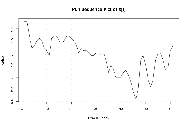
| Dataseries X: | |||||||||||||||||||||||||||||||||||||||||||||||||||||||||||||||||
9.3 9.3 8.7 8.2 8.3 8.5 8.6 8.5 8.2 8.1 7.9 8.6 8.7 8.7 8.5 8.4 8.5 8.7 8.7 8.6 8.5 8.3 8 8.2 8.1 8.1 8 7.9 7.9 8 8 7.9 8 7.7 7.2 7.5 7.3 7 7 7 7.2 7.3 7.1 6.8 6.4 6.1 6.5 7.7 7.9 7.5 6.9 6.6 6.9 7.7 8 8 7.7 7.3 7.4 8.1 8.3 | |||||||||||||||||||||||||||||||||||||||||||||||||||||||||||||||||
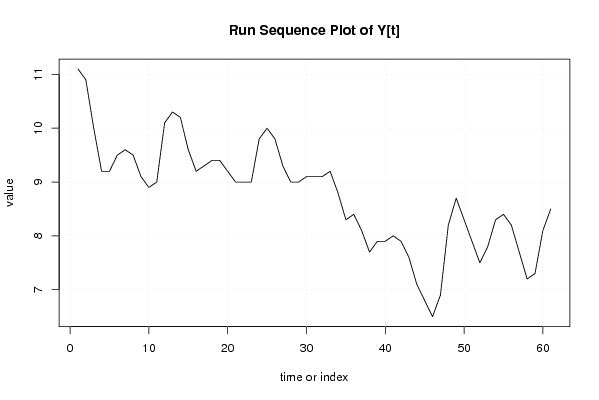
| Dataseries Y: | |||||||||||||||||||||||||||||||||||||||||||||||||||||||||||||||||
11,1 10,9 10,0 9,2 9,2 9,5 9,6 9,5 9,1 8,9 9,0 10,1 10,3 10,2 9,6 9,2 9,3 9,4 9,4 9,2 9,0 9,0 9,0 9,8 10,0 9,8 9,3 9,0 9,0 9,1 9,1 9,1 9,2 8,8 8,3 8,4 8,1 7,7 7,9 7,9 8,0 7,9 7,6 7,1 6,8 6,5 6,9 8,2 8,7 8,3 7,9 7,5 7,8 8,3 8,4 8,2 7,7 7,2 7,3 8,1 8,5 | |||||||||||||||||||||||||||||||||||||||||||||||||||||||||||||||||
Tables (Output of Computation) | |||||||||||||||||||||||||||||||||||||||||||||||||||||||||||||||||
| |||||||||||||||||||||||||||||||||||||||||||||||||||||||||||||||||
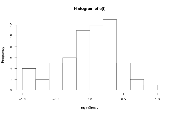
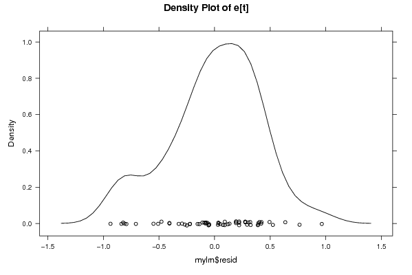
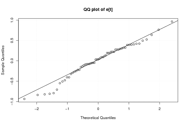
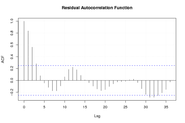
Figures (Output of Computation) | |||||||||||||||||||||||||||||||||||||||||||||||||||||||||||||||||
Input Parameters & R Code | |||||||||||||||||||||||||||||||||||||||||||||||||||||||||||||||||
| Parameters (Session): | |||||||||||||||||||||||||||||||||||||||||||||||||||||||||||||||||
| par1 = 0 ; par2 = 36 ; | |||||||||||||||||||||||||||||||||||||||||||||||||||||||||||||||||
| Parameters (R input): | |||||||||||||||||||||||||||||||||||||||||||||||||||||||||||||||||
| par1 = 0 ; par2 = 36 ; | |||||||||||||||||||||||||||||||||||||||||||||||||||||||||||||||||
| R code (references can be found in the software module): | |||||||||||||||||||||||||||||||||||||||||||||||||||||||||||||||||
par1 <- as.numeric(par1) | |||||||||||||||||||||||||||||||||||||||||||||||||||||||||||||||||