Repository of Reproducible Computations

Free Statistics

of Irreproducible Research!

Author's title

Author

*The author of this computation has been verified*

R Software Module

rwasp_edabi.wasp

Title produced by software

Bivariate Explorative Data Analysis

Date of computation

Wed, 04 Nov 2009 04:34:29 -0700

Cite this page as follows

Statistical Computations at FreeStatistics.org, Office for Research Development and Education, URL https://freestatistics.org/blog/index.php?v=date/2009/Nov/04/t1257334595dkyiws25odngdsv.htm/, Retrieved Mon, 29 Apr 2024 12:02:57 +0000

Statistical Computations at FreeStatistics.org, Office for Research Development and Education, URL https://freestatistics.org/blog/index.php?pk=53566, Retrieved Mon, 29 Apr 2024 12:02:57 +0000

QR Codes:

Paste this QR Code to cite your computation.

Original text written by user:

IsPrivate?

No (this computation is public)

User-defined keywords

WS 5 (Et inY en E�t in X)

Estimated Impact

184

Family? (F = Feedback message, R = changed R code, M = changed R Module, P = changed Parameters, D = changed Data)

-     [Bivariate Data Series] [Bivariate dataset] [2008-01-05 23:51:08] [74be16979710d4c4e7c6647856088456]
- RMPD  [Bivariate Explorative Data Analysis] [] [2009-10-28 15:16:32] [5482608004c1d7bbf873930172393a2d]
-    D    [Bivariate Explorative Data Analysis] [] [2009-10-28 16:44:36] [5482608004c1d7bbf873930172393a2d]
- RMPD      [Trivariate Scatterplots] [] [2009-11-03 17:57:36] [5482608004c1d7bbf873930172393a2d]
- RMPD        [Bivariate Explorative Data Analysis] [] [2009-11-03 18:33:00] [5482608004c1d7bbf873930172393a2d]
-    D            [Bivariate Explorative Data Analysis] [Workshop 5 Bivari...] [2009-11-04 11:34:29] [e2f800c9186517d2e5c4a809848912a7] [Current]

Feedback Forum

Post a new message

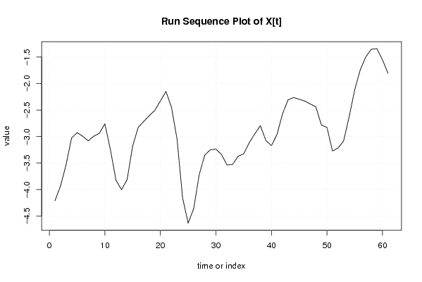
Dataseries X:

Download CSV

Histogram

Boxplots

-4.213500441
-3.935935693
-3.536894327
-3.026635334
-2.926635334
-2.992982456
-3.08176483
-2.992982456
-2.93785296
-2.760288212
-3.249070586
-3.825676701
-4.003241449
-3.814459075
-3.18176483
-2.826635334
-2.715417708
-2.604200082
-2.504200082
-2.326635334
-2.149070586
-2.449070586
-3.049070586
-4.159329578
-4.636894327
-4.359329578
-3.715417708
-3.349070586
-3.249070586
-3.23785296
-3.33785296
-3.53785296
-3.526635334
-3.371505838
-3.327593967
-3.116376341
-2.950029219
-2.794899723
-3.072464471
-3.172464471
-2.961246845
-2.572464471
-2.306117349
-2.262205478
-2.295858356
-2.329511234
-2.38464073
-2.438811593
-2.782723464
-2.827593967
-3.272464471
-3.217334975
-3.083682097
-2.627593967
-2.116376341
-1.738811593
-1.494899723
-1.350987852
-1.339770226
-1.550029219
-1.805158715

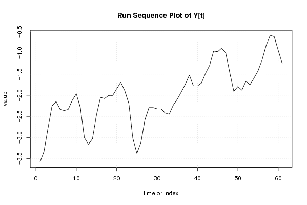
Dataseries Y:

Download CSV

Histogram

-3.585860839
-3.329201771
-2.774235967
-2.247599696
-2.147599696
-2.332588297
-2.360917831
-2.332588297
-2.119270162
-1.962611095
-2.290940628
-3.0025655
-3.159224568
-3.030895034
-2.460917831
-2.047599696
-2.07592923
-2.004258764
-2.004258764
-1.847599696
-1.690940628
-1.890940628
-2.190940628
-3.017576899
-3.374235967
-3.117576899
-2.57592923
-2.290940628
-2.290940628
-2.319270162
-2.319270162
-2.419270162
-2.447599696
-2.234281561
-2.092633892
-1.920963426
-1.735974824
-1.522656689
-1.779315756
-1.779315756
-1.70764529
-1.479315756
-1.294327155
-0.952679486
-0.967690884
-0.882702283
-0.996020418
-1.464304358
-1.905952027
-1.792633892
-1.879315756
-1.665997621
-1.750986223
-1.592633892
-1.420963426
-1.164304358
-0.822656689
-0.58100902
-0.609338554
-0.935974824
-1.249292959

Summary of computational transaction
Raw Input	view raw input (R code)
Raw Output	view raw output of R engine
Computing time	14 seconds
R Server	'Gwilym Jenkins' @ 72.249.127.135

\begin{tabular}{lllllllll}
\hline
Summary of computational transaction \tabularnewline
Raw Input & view raw input (R code)  \tabularnewline
Raw Output & view raw output of R engine  \tabularnewline
Computing time & 14 seconds \tabularnewline
R Server & 'Gwilym Jenkins' @ 72.249.127.135 \tabularnewline
\hline
\end{tabular}
%Source: https://freestatistics.org/blog/index.php?pk=53566&T=0

[TABLE]
[ROW][C]Summary of computational transaction[/C][/ROW]
[ROW][C]Raw Input[/C][C]view raw input (R code) [/C][/ROW]
[ROW][C]Raw Output[/C][C]view raw output of R engine [/C][/ROW]
[ROW][C]Computing time[/C][C]14 seconds[/C][/ROW]
[ROW][C]R Server[/C][C]'Gwilym Jenkins' @ 72.249.127.135[/C][/ROW]
[/TABLE]
Source: https://freestatistics.org/blog/index.php?pk=53566&T=0

Globally Unique Identifier (entire table): ba.freestatistics.org/blog/index.php?pk=53566&T=0

As an alternative you can also use a QR Code:

The GUIDs for individual cells are displayed in the table below:

Summary of computational transaction
Raw Input	view raw input (R code)
Raw Output	view raw output of R engine
Computing time	14 seconds
R Server	'Gwilym Jenkins' @ 72.249.127.135

Model: Y[t] = c + b X[t] + e[t]
c	0.601350348816443
b	0.883365504377919

\begin{tabular}{lllllllll}
\hline
Model: Y[t] = c + b X[t] + e[t] \tabularnewline
c & 0.601350348816443 \tabularnewline
b & 0.883365504377919 \tabularnewline
\hline
\end{tabular}
%Source: https://freestatistics.org/blog/index.php?pk=53566&T=1

[TABLE]
[ROW][C]Model: Y[t] = c + b X[t] + e[t][/C][/ROW]
[ROW][C]c[/C][C]0.601350348816443[/C][/ROW]
[ROW][C]b[/C][C]0.883365504377919[/C][/ROW]
[/TABLE]
Source: https://freestatistics.org/blog/index.php?pk=53566&T=1

Globally Unique Identifier (entire table): ba.freestatistics.org/blog/index.php?pk=53566&T=1

As an alternative you can also use a QR Code:

The GUIDs for individual cells are displayed in the table below:

Model: Y[t] = c + b X[t] + e[t]
c	0.601350348816443
b	0.883365504377919

Descriptive Statistics about e[t]
# observations	61
minimum	-0.465150245555893
Q1	-0.229648526947825
median	-0.0221740998550922
mean	-4.18093241038959e-17
Q3	0.142640045281525
maximum	0.574734763127151

\begin{tabular}{lllllllll}
\hline
Descriptive Statistics about e[t] \tabularnewline
# observations & 61 \tabularnewline
minimum & -0.465150245555893 \tabularnewline
Q1 & -0.229648526947825 \tabularnewline
median & -0.0221740998550922 \tabularnewline
mean & -4.18093241038959e-17 \tabularnewline
Q3 & 0.142640045281525 \tabularnewline
maximum & 0.574734763127151 \tabularnewline
\hline
\end{tabular}
%Source: https://freestatistics.org/blog/index.php?pk=53566&T=2

[TABLE]
[ROW][C]Descriptive Statistics about e[t][/C][/ROW]
[ROW][C]# observations[/C][C]61[/C][/ROW]
[ROW][C]minimum[/C][C]-0.465150245555893[/C][/ROW]
[ROW][C]Q1[/C][C]-0.229648526947825[/C][/ROW]
[ROW][C]median[/C][C]-0.0221740998550922[/C][/ROW]
[ROW][C]mean[/C][C]-4.18093241038959e-17[/C][/ROW]
[ROW][C]Q3[/C][C]0.142640045281525[/C][/ROW]
[ROW][C]maximum[/C][C]0.574734763127151[/C][/ROW]
[/TABLE]
Source: https://freestatistics.org/blog/index.php?pk=53566&T=2

Globally Unique Identifier (entire table): ba.freestatistics.org/blog/index.php?pk=53566&T=2

As an alternative you can also use a QR Code:

The GUIDs for individual cells are displayed in the table below:

Descriptive Statistics about e[t]
# observations	61
minimum	-0.465150245555893
Q1	-0.229648526947825
median	-0.0221740998550922
mean	-4.18093241038959e-17
Q3	0.142640045281525
maximum	0.574734763127151

Figure 1

PNG link

Postscript link

PDF link

Figure 2

PNG link

Postscript link

PDF link

Figure 3

PNG link

Postscript link

PDF link

Figure 4

PNG link

Postscript link

PDF link

Figure 5

PNG link

Postscript link

PDF link

Figure 6

PNG link

Postscript link

PDF link

Figure 7

PNG link

Postscript link

PDF link

Figure 8

PNG link

Postscript link

PDF link

Parameters (Session):

par1 = 0 ; par2 = 36 ;

Parameters (R input):

par1 = 0 ; par2 = 36 ;

R code (references can be found in the software module):

par1 <- as.numeric(par1)
par2 <- as.numeric(par2)
x <- as.ts(x)
y <- as.ts(y)
mylm <- lm(y~x)
cbind(mylm$resid)
library(lattice)
bitmap(file='pic1.png')
plot(y,type='l',main='Run Sequence Plot of Y[t]',xlab='time or index',ylab='value')
grid()
dev.off()
bitmap(file='pic1a.png')
plot(x,type='l',main='Run Sequence Plot of X[t]',xlab='time or index',ylab='value')
grid()
dev.off()
bitmap(file='pic1b.png')
plot(x,y,main='Scatter Plot',xlab='X[t]',ylab='Y[t]')
grid()
dev.off()
bitmap(file='pic1c.png')
plot(mylm$resid,type='l',main='Run Sequence Plot of e[t]',xlab='time or index',ylab='value')
grid()
dev.off()
bitmap(file='pic2.png')
hist(mylm$resid,main='Histogram of e[t]')
dev.off()
bitmap(file='pic3.png')
if (par1 > 0)
{
densityplot(~mylm$resid,col='black',main=paste('Density Plot of e[t]   bw = ',par1),bw=par1)
} else {
densityplot(~mylm$resid,col='black',main='Density Plot of e[t]')
}
dev.off()
bitmap(file='pic4.png')
qqnorm(mylm$resid,main='QQ plot of e[t]')
qqline(mylm$resid)
grid()
dev.off()
if (par2 > 0)
{
bitmap(file='pic5.png')
acf(mylm$resid,lag.max=par2,main='Residual Autocorrelation Function')
grid()
dev.off()
}
summary(x)
load(file='createtable')
a<-table.start()
a<-table.row.start(a)
a<-table.element(a,'Model: Y[t] = c + b X[t] + e[t]',2,TRUE)
a<-table.row.end(a)
a<-table.row.start(a)
a<-table.element(a,'c',1,TRUE)
a<-table.element(a,mylm$coeff[[1]])
a<-table.row.end(a)
a<-table.row.start(a)
a<-table.element(a,'b',1,TRUE)
a<-table.element(a,mylm$coeff[[2]])
a<-table.row.end(a)
a<-table.end(a)
table.save(a,file='mytable.tab')
a<-table.start()
a<-table.row.start(a)
a<-table.element(a,'Descriptive Statistics about e[t]',2,TRUE)
a<-table.row.end(a)
a<-table.row.start(a)
a<-table.element(a,'# observations',header=TRUE)
a<-table.element(a,length(mylm$resid))
a<-table.row.end(a)
a<-table.row.start(a)
a<-table.element(a,'minimum',header=TRUE)
a<-table.element(a,min(mylm$resid))
a<-table.row.end(a)
a<-table.row.start(a)
a<-table.element(a,'Q1',header=TRUE)
a<-table.element(a,quantile(mylm$resid,0.25))
a<-table.row.end(a)
a<-table.row.start(a)
a<-table.element(a,'median',header=TRUE)
a<-table.element(a,median(mylm$resid))
a<-table.row.end(a)
a<-table.row.start(a)
a<-table.element(a,'mean',header=TRUE)
a<-table.element(a,mean(mylm$resid))
a<-table.row.end(a)
a<-table.row.start(a)
a<-table.element(a,'Q3',header=TRUE)
a<-table.element(a,quantile(mylm$resid,0.75))
a<-table.row.end(a)
a<-table.row.start(a)
a<-table.element(a,'maximum',header=TRUE)
a<-table.element(a,max(mylm$resid))
a<-table.row.end(a)
a<-table.end(a)
table.save(a,file='mytable.tab')

Free Statistics

Description of Statistical Computation

Tree of Dependent Computations

Dataset

Tables (Output of Computation)

Figures (Output of Computation)

Input Parameters & R Code