Free Statistics
of Irreproducible Research!
Description of Statistical Computation | |||||||||||||||||||||||||||||||||||||||||||||||||||||
|---|---|---|---|---|---|---|---|---|---|---|---|---|---|---|---|---|---|---|---|---|---|---|---|---|---|---|---|---|---|---|---|---|---|---|---|---|---|---|---|---|---|---|---|---|---|---|---|---|---|---|---|---|---|
| Author's title | |||||||||||||||||||||||||||||||||||||||||||||||||||||
| Author | *The author of this computation has been verified* | ||||||||||||||||||||||||||||||||||||||||||||||||||||
| R Software Module | rwasp_edauni.wasp | ||||||||||||||||||||||||||||||||||||||||||||||||||||
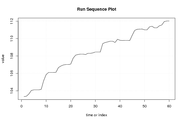
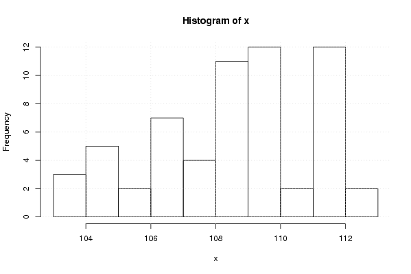
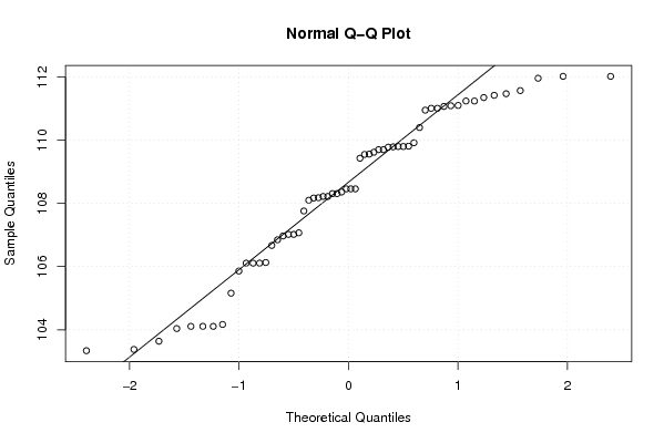
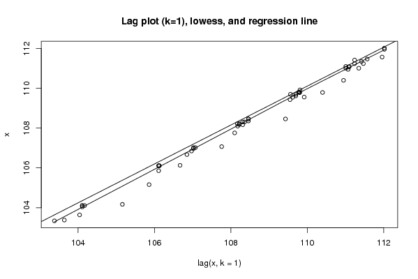
| Title produced by software | Univariate Explorative Data Analysis | ||||||||||||||||||||||||||||||||||||||||||||||||||||
| Date of computation | Wed, 04 Nov 2009 05:01:28 -0700 | ||||||||||||||||||||||||||||||||||||||||||||||||||||
| Cite this page as follows | Statistical Computations at FreeStatistics.org, Office for Research Development and Education, URL https://freestatistics.org/blog/index.php?v=date/2009/Nov/04/t1257336120yyxg2cqhb3jnqsb.htm/, Retrieved Mon, 29 Apr 2024 10:10:40 +0000 | ||||||||||||||||||||||||||||||||||||||||||||||||||||
| Statistical Computations at FreeStatistics.org, Office for Research Development and Education, URL https://freestatistics.org/blog/index.php?pk=53578, Retrieved Mon, 29 Apr 2024 10:10:40 +0000 | |||||||||||||||||||||||||||||||||||||||||||||||||||||
| QR Codes: | |||||||||||||||||||||||||||||||||||||||||||||||||||||
|
| |||||||||||||||||||||||||||||||||||||||||||||||||||||
| Original text written by user: | |||||||||||||||||||||||||||||||||||||||||||||||||||||
| IsPrivate? | No (this computation is public) | ||||||||||||||||||||||||||||||||||||||||||||||||||||
| User-defined keywords | |||||||||||||||||||||||||||||||||||||||||||||||||||||
| Estimated Impact | 139 | ||||||||||||||||||||||||||||||||||||||||||||||||||||
Tree of Dependent Computations | |||||||||||||||||||||||||||||||||||||||||||||||||||||
| Family? (F = Feedback message, R = changed R code, M = changed R Module, P = changed Parameters, D = changed Data) | |||||||||||||||||||||||||||||||||||||||||||||||||||||
| - [Notched Boxplots] [3/11/2009] [2009-11-02 21:10:41] [b98453cac15ba1066b407e146608df68] - D [Notched Boxplots] [ws 6 1] [2009-11-04 11:54:28] [6e4e01d7eb22a9f33d58ebb35753a195] - RMPD [Univariate Explorative Data Analysis] [ws 6 kla] [2009-11-04 11:57:24] [6e4e01d7eb22a9f33d58ebb35753a195] - [Univariate Explorative Data Analysis] [ws 6 sto] [2009-11-04 11:59:43] [6e4e01d7eb22a9f33d58ebb35753a195] - D [Univariate Explorative Data Analysis] [ws 6 sch] [2009-11-04 12:01:28] [2e4ef2c1b76db9b31c0a03b96e94ad77] [Current] - D [Univariate Explorative Data Analysis] [ws 6 totpr] [2009-11-04 12:02:45] [6e4e01d7eb22a9f33d58ebb35753a195] | |||||||||||||||||||||||||||||||||||||||||||||||||||||
| Feedback Forum | |||||||||||||||||||||||||||||||||||||||||||||||||||||
Post a new message | |||||||||||||||||||||||||||||||||||||||||||||||||||||
Dataset | |||||||||||||||||||||||||||||||||||||||||||||||||||||
| Dataseries X: | |||||||||||||||||||||||||||||||||||||||||||||||||||||
103,34 103,38 103,64 104,04 104,11 104,11 104,11 104,17 105,16 105,86 106,11 106,11 106,11 106,13 106,67 106,85 106,97 107,02 107,02 107,07 107,76 108,10 108,18 108,22 108,22 108,17 108,31 108,31 108,36 108,46 108,46 108,46 109,43 109,55 109,62 109,70 109,70 109,56 109,92 109,81 109,78 109,80 109,80 109,79 110,40 110,95 111,07 111,09 111,10 111,01 111,01 111,35 111,42 111,24 111,24 111,47 111,57 111,96 112,02 112,02 | |||||||||||||||||||||||||||||||||||||||||||||||||||||
Tables (Output of Computation) | |||||||||||||||||||||||||||||||||||||||||||||||||||||
| |||||||||||||||||||||||||||||||||||||||||||||||||||||
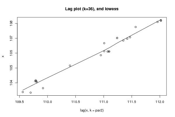
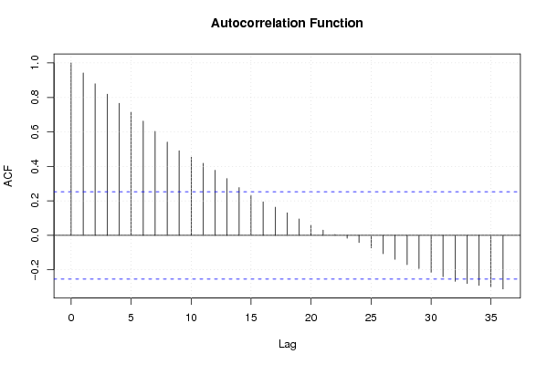
Figures (Output of Computation) | |||||||||||||||||||||||||||||||||||||||||||||||||||||
Input Parameters & R Code | |||||||||||||||||||||||||||||||||||||||||||||||||||||
| Parameters (Session): | |||||||||||||||||||||||||||||||||||||||||||||||||||||
| par1 = 0 ; par2 = 36 ; | |||||||||||||||||||||||||||||||||||||||||||||||||||||
| Parameters (R input): | |||||||||||||||||||||||||||||||||||||||||||||||||||||
| par1 = 0 ; par2 = 36 ; | |||||||||||||||||||||||||||||||||||||||||||||||||||||
| R code (references can be found in the software module): | |||||||||||||||||||||||||||||||||||||||||||||||||||||
par1 <- as.numeric(par1) | |||||||||||||||||||||||||||||||||||||||||||||||||||||