Free Statistics
of Irreproducible Research!
Description of Statistical Computation | |||||||||||||||||||||
|---|---|---|---|---|---|---|---|---|---|---|---|---|---|---|---|---|---|---|---|---|---|
| Author's title | |||||||||||||||||||||
| Author | *The author of this computation has been verified* | ||||||||||||||||||||
| R Software Module | rwasp_cloud.wasp | ||||||||||||||||||||
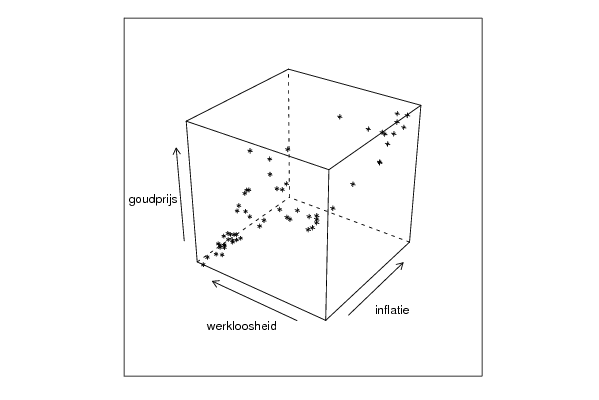
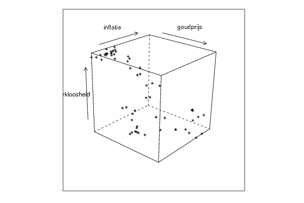
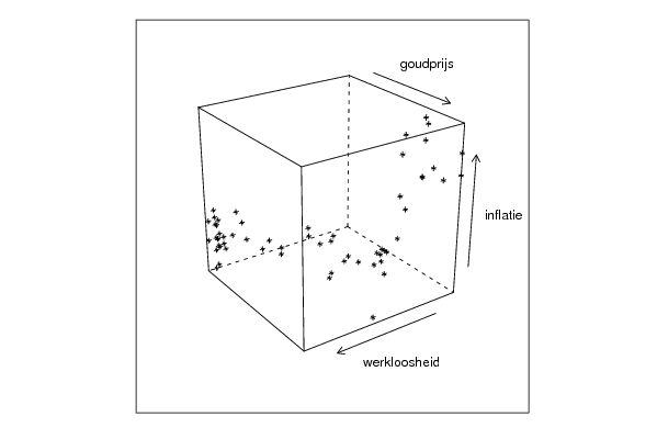
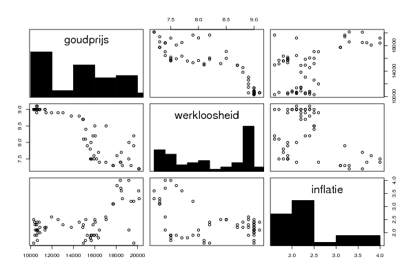
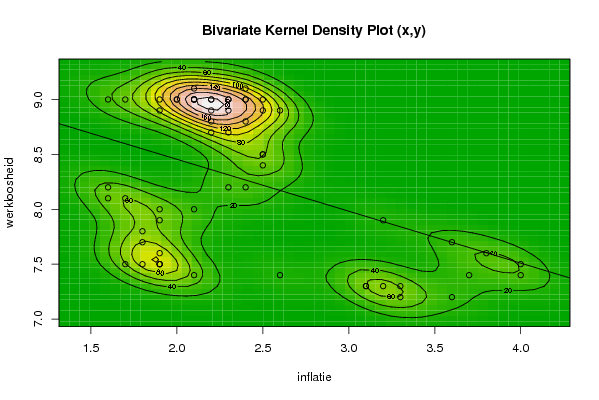
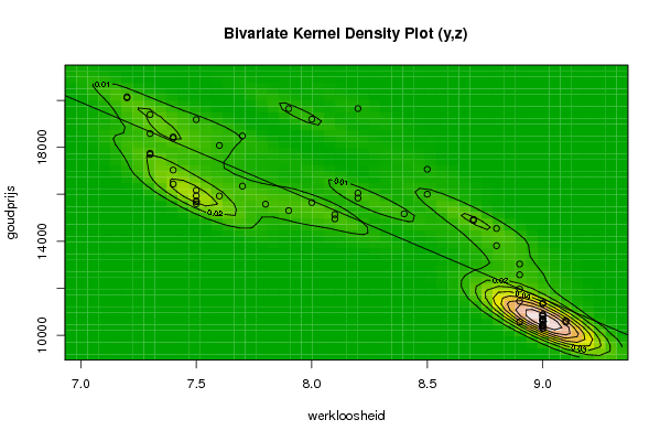
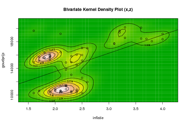
| Title produced by software | Trivariate Scatterplots | ||||||||||||||||||||
| Date of computation | Wed, 04 Nov 2009 07:48:05 -0700 | ||||||||||||||||||||
| Cite this page as follows | Statistical Computations at FreeStatistics.org, Office for Research Development and Education, URL https://freestatistics.org/blog/index.php?v=date/2009/Nov/04/t12573461814vw5lnkghr2yo0d.htm/, Retrieved Mon, 29 Apr 2024 12:35:58 +0000 | ||||||||||||||||||||
| Statistical Computations at FreeStatistics.org, Office for Research Development and Education, URL https://freestatistics.org/blog/index.php?pk=53601, Retrieved Mon, 29 Apr 2024 12:35:58 +0000 | |||||||||||||||||||||
| QR Codes: | |||||||||||||||||||||
|
| |||||||||||||||||||||
| Original text written by user: | |||||||||||||||||||||
| IsPrivate? | No (this computation is public) | ||||||||||||||||||||
| User-defined keywords | |||||||||||||||||||||
| Estimated Impact | 125 | ||||||||||||||||||||
Tree of Dependent Computations | |||||||||||||||||||||
| Family? (F = Feedback message, R = changed R code, M = changed R Module, P = changed Parameters, D = changed Data) | |||||||||||||||||||||
| - [Univariate Data Series] [] [2009-10-12 17:39:23] [74be16979710d4c4e7c6647856088456] - RMPD [Trivariate Scatterplots] [cs.shw.ws5.v1] [2009-11-04 14:48:05] [47f146dd9fb230449e079c6cbc92f5f5] [Current] | |||||||||||||||||||||
| Feedback Forum | |||||||||||||||||||||
Post a new message | |||||||||||||||||||||
Dataset | |||||||||||||||||||||
| Dataseries X: | |||||||||||||||||||||
1,9 1,6 1,7 2 2,5 2,4 2,3 2,3 2,1 2,4 2,2 2,4 1,9 2,1 2,1 2,1 2 2,1 2,2 2,2 2,6 2,5 2,3 2,2 2,4 2,3 2,2 2,5 2,5 2,5 2,4 2,3 1,7 1,6 1,9 1,9 1,8 1,8 1,9 1,9 1,9 1,9 1,8 1,7 2,1 2,6 3,1 3,1 3,2 3,3 3,6 3,3 3,7 4 4 3,8 3,6 3,2 2,1 1,6 | |||||||||||||||||||||
| Dataseries Y: | |||||||||||||||||||||
8,9 9 9 9 9 9 9 9 9 9 9 9,1 9 9 9,1 9 9 9 9 8,9 8,9 8,9 8,9 8,8 8,8 8,7 8,7 8,5 8,5 8,4 8,2 8,2 8,1 8,1 8 7,9 7,8 7,7 7,6 7,5 7,5 7,5 7,5 7,5 7,4 7,4 7,3 7,3 7,3 7,2 7,2 7,3 7,4 7,4 7,5 7,6 7,7 7,9 8 8,2 | |||||||||||||||||||||
| Dataseries Z: | |||||||||||||||||||||
10570 10297 10635 10872 10296 10383 10431 10574 10653 10805 10872 10625 10407 10463 10556 10646 10702 11353 11346 11451 11964 12574 13031 13812 14544 14931 14886 16005 17064 15168 16050 15839 15137 14954 15648 15305 15579 16348 15928 16171 15937 15713 15594 15683 16438 17032 17696 17745 19394 20148 20108 18584 18441 18391 19178 18079 18483 19644 19195 19650 | |||||||||||||||||||||
Tables (Output of Computation) | |||||||||||||||||||||
| |||||||||||||||||||||
Figures (Output of Computation) | |||||||||||||||||||||
Input Parameters & R Code | |||||||||||||||||||||
| Parameters (Session): | |||||||||||||||||||||
| par1 = 50 ; par2 = 50 ; par3 = Y ; par4 = Y ; par5 = inflatie ; par6 = werkloosheid ; par7 = goudprijs ; | |||||||||||||||||||||
| Parameters (R input): | |||||||||||||||||||||
| par1 = 50 ; par2 = 50 ; par3 = Y ; par4 = Y ; par5 = inflatie ; par6 = werkloosheid ; par7 = goudprijs ; | |||||||||||||||||||||
| R code (references can be found in the software module): | |||||||||||||||||||||
x <- array(x,dim=c(length(x),1)) | |||||||||||||||||||||